***START OF THE PROJECT GUTENBERG EBOOK DEFINITION & REALITY IN THE GENERAL THEORY OF POLITICAL ECONOMY***

Definition & Reality
in the
General Theory of Political Economy

Thomas Colignatus

Dutch University Press

Samuel van Houten Genootschap

This text is made available by the copyright owner as an etext for the Project Gutenberg (see http://www.gutenberg.org). The Project Gutenberg header specifies under what general conditions the book may be distributed while associated with the Project Gutenberg trademark. Additional conditions are: (a) No commercial use or resale of the etext is allowed, (b) Hardcopy prints are to be acquired at the publisher Dutch University Press (see http://www.rozenbergps.com and ISBN 90-3619-172-6) or their designated partners. Please note that the etext uses HTML so that the etext layout will differ significantly from the official layout.

2^nd edition, January 2005
(The first edition was in March & June 2000)

Colignatus is the preferred name of Thomas Cool in science.

Lawful exceptions excluded, nothing of this publication may be copied or published by means of print, photocopy, microfilm, electronics or otherwise, unless a written permit has been given by the lawful owners of the copyright, and this also holds for whole or partial reworkings.

Behoudens uitzondering door de wet gesteld mag zonder schriftelijke toestemming van de rechthebbende(n) op het auteursrecht niets uit deze uitgave worden verveelvoudigd en/of openbaar gemaakt door middel van druk, fotokopie, microfilm, electronica of anderszins, hetgeen ook van toepassing is op gehele of gedeeltelijke bewerking.

Published by

Dutch University Press
in association with Purdue University Press, West Lafayette, Indiana, U.S.A.
& Rozenberg Publishers, Amsterdam, The Netherlands.
Bloemgracht 82hs, 1015 TM Amsterdam, http://www.rozenbergps.com
Tel. +31-(0)20-6255429, fax +31-(0)20-6203395, email info@rozenbergps.com

Supported by

Samuel van Houten Genootschap

Wetenschappelijk bureau van het Sociaal Liberaal Forum
Scientific bureau of the Social Liberal Forum
P.O. Box 78, 2501 CB The Hague, Holland
Tel +31-(0)70-3555404 Fax +31-(0)-842113307 Giro 450623

ISBN 90-3619-172-6

JEL A00

Nederlandse uniforme genre indeling (NUGI) 681, 654 & 691

CIP-GEGEVENS KONINKLIJKE BIBLIOTHEEK ’S-GRAVENHAGE

Prologue

The basic idea of this book is that Keynes’s General Theory is generalised even further by including endogenous government in the model, so that we arrive at a truly general Political Economy. The world had the Great Depression 1930-1940 and has the Great Stagflation 1970-today and by including ‘stagnation in economic policy making’ in our analysis we find a better explanation. The general theory also advises a democracy to create an Economic Supreme Court as a separate constitutional power, next to the Legislative, Executive and Judicial branches.

This book is primarily directed at my fellow economists and it primarily gives theory and stylized facts. The colleagues will specifically have to understand the ‘Definition & Reality methodology’ before they will appreciate that my analysis is scientifically warranted. Much work remains to be done in practical research. And much work remains to be done by the other professions.

Since the current imbalance of powers has many victims, it may be hoped, none the less, that the parliaments of our democratic nations investigate the issue too, so that there is more hope for improvement in their living conditions. Parliaments should do as Alfred Marshall (1890, 1947:3) wrote:

“Now at least we are setting ourselves seriously to inquire whether it is necessary that there should be any so-called ‘lower-classes’ at all: that is, whether there need be large numbers of people doomed from their birth to hard work in order to provide for others the requisites of a refined and cultured life; while they themselves are prevented by their poverty and toil from having any share or part in that life.”

Books are more stimulating and more enjoyable to read if they are guided by questions and if they cause questions themselves. This book has been written in the style that it provides answers and thus it must be feared to be a dull read. It is too late to change that style. However, some questions are: (1) How is it possible that Europe has an unemployment of about 10% for more than three decades now, and the USA the mirror image of poverty ? (2) Can we really trust our governments ?

With this book ends a project that basically started with the Fall of the Berlin Wall in 1989. My hope is that this book contributes to the fall of some other walls, i.e. the intangible mental ones, consisting of perceptions and conventions - but equally confining.

Contents in Brief

Book I Introduction 11

Book II Trias Politica and Economic Supreme Court 16

Book III Economics ‘as usual’ 36

Book IV Presentations for the general public 60

Book V Methodology: Definition & Reality 69

Book VI Structural models 87

Book VII Social Choice 158

Book VIII Supportive notions 186

Book IX Reduced form 198

Book X Conclusions 216

Appendices 266

The symbol ° is used to indicate market clearing equilibrium (and possibly expectational). The symbol * or E[.]is used for expectations and expectational equilibrium (and possibly market clearing). The symbol °* is used for both, and ^· for the one or the other (and possibly both).

Contents

Book I Introduction 11

1. Order of presentation 11

2. The general theory 11

3. Methodology 14

Book II Trias Politica and Economic Supreme Court 16

4. The Trias Politica 16

5. The economic record of the 20^th century 18

6. An Economic Supreme Court 24

7. Position of the Court in economic theory 26

8. The record of economics itself 26

9. Economics ‘as usual’ and its inadequacy 30

10. Four empirical cases 32

11. The moral imperative 33

Book III Economics ‘as usual’ 36

12. Introduction 36

Stylized history 38

Structure of the argument 41

The difference that it means 42

13. Unemployment via taxes and minimum wage 43

The earnings distribution 44

Analysing the minimum wage 44

The Tax Void 47

Cause of the Tax Void 48

Development of the Tax Void 51

Marginal tax rate & VAT 53

Marginal tax rate & dynamics 54

Spillover and domino effects 56

Diagnosis and Therapy 56

Stagflation resolved 57

14. The 1974 Duisenberg disaster 59

Book IV Presentations for the general public 60

15. Unemployment solved ! 60

16. Enable Russia to help itself 64

Parallel 64

Risk not chance 65

Internal not external 65

Conclusion 66

17. Will the West repeat Versailles ? 66

Book V Methodology: Definition & Reality 69

18. How to check ? 69

19. Dealing economically with concepts 70

Maximising information power 70

Pythagoras and the circle 73

Falsification 76

Determinism and free will 78

From stylized fact to definition 82

Relating to Hicks 1983 83

20. Structural and reduced form 84

21. Direct application to the Economic Supreme Court 85

22. Methodological summary 85

Book VI Structural models 87

23. A textbook macro-economic model 87

The IS-LM model 87

The production function 89

Dynamics versus statics 90

Phillipscurve 90

Macro-economic interactions 91

24. Heterogeneity and nonlinear taxation 92

Heterogeneity versus homogeneity 92

Nonlinear versus proportional taxation 93

Some literature 93

25. Summary of current views 94

A simple view 94

A complex view 96

Efficiency wages intermezzo 96

A more sophisticated view 97

Confusions 98

26. Heterogeneous labour 99

Dromedary supply 99

Dutch income distribution data 100

Definitions and formulas 102

Amendment to the textbook model on the Phillipscurve 106

27. Subsistence 106

Definitions 107

Economic literature 109

Types of indexation 109

Formal development 110

28. Phillipscurve 115

Concepts 115

A homogeneous Phillipscurve 118

On expectations 121

Heterogeneous Phillipscurves 122

More factors that cause a shift 122

Crowding out 123

Poverty 124

The submarket Phillipscurves 125

Shifting back 125

29. Tax basics 126

Taxes and premiums 126

Common structure 127

Nonlinear tax function 128

Exemption 129

The marginal rate 140

Balanced growth 143

Off balanced growth 144

30. Dynamic curvature of the tax wedge 145

Introduction 145

Formulas 145

Graphs 147

31. Differential impact of the minimum wage on exposed and sheltered sectors 149

Introduction 149

Model 151

Graphs 152

Tables 154

Conclusion 155

32. Dynamic optimality 155

The Phillipscurve revisited 155

Investment, growth and productivity 156

Book VII Social Choice 158

33. Introduction 158

34. The solution to Arrow’s difficulty in social choice 159

Introduction 159

Basic concepts 162

Restatement of Arrow’s Theorem 165

A note on the name of APDM 167

A lemma 167

Rejection of the Arrow Moral Claim (AMC) 168

Rejection of the Arrow Reasonableness Claim (ARC) 168

Selection of the culprit axiom. 169

Examples of consistent constitutions 170

A reappraisal of the literature 170

Conclusion 172

Addendum: Sen’s restatement in “Development as freedom” 172

Addendum: Mas-colell, Whinston and Green, “Microeconomic Theory” 175

35. Without time, no morality 175

Introduction 175

Control of natural forces in the social process 176

Three traditional methods 177

Borda Fixed point 178

Relation to Saari’s work 179

Pareto 182

A note on cheating 182

Conclusion 183

36. Some notes on ethics 183

Book VIII Supportive notions 186

37. On the nature and significance of a free lunch 186

Some quotes 186

Consumers surplus 187

Economic growth 188

Conclusion 192

38. Proper definitions for uncertainty and risk 192

Uncertainty 192

Risk 193

Example 195

Wrong use in economics 1921-2005 196

Book IX Reduced form 198

39. The possibility of full employment in the welfare state 198

Introduction 198

Stylized facts 198

Concepts 199

The theorem 201

Graphical presentation 205

40. The possibility of co-ordination 206

Stylized facts 206

Concepts 207

The special theorem 211

The general theorem 213

On the interaction of the reduced form theorems 214

Book I
Introduction

1. Order of presentation

The basic idea of this book is that Keynes’s General Theory is generalised even further by including endogenous government in the model so that we arrive at a truly general Political Economy. The argument can be presented in a top-down fashion, for example by repeating the IS-LM model before the amendments are introduced. This order appears to be uninviting and therefor the argument is presented in a bottom-up fashion. We better discuss the amendments before we look at the consequences for theory as a whole. We start with the new economic synthesis and the argument for the Economic Supreme Court, since these motivate the book.

2. The general theory

Political Economy is the science of the management of the state. More in general, ‘economics’ is Greekish for ‘management theory’. [1] Marshall already explained that ‘economics’ is wider than ‘political economy’, see his “Principles of economics” (1947:43). The proper definitions are:

· Economics ‘in a narrow sense’ puts the approach, methods and tools, of the discipline central, and looks at a variety of subjects.

· Political Economy puts the subject, the management of the state, central.

· Economics ‘in a broad sense’ joins the ‘narrow sense’ and Political Economy.

One way to view these distinctions is to visualize a matrix with the sciences in the rows and the subjects in the columns. The common economist may to some extent neglect the inputs of the other disciplines, but the political economist must draw on the resources of philosophy, history, law, sociology, politicology, social psychology, biology, physics and so on. [2] Political Economy is, just by definition, the study that tries to integrate all human knowledge about the management of the state. Political Economy is, in that respect, the proper continuation of ancient philosophy on that subject matter.

Confusions easily arise when these definitions are not understood. [3]

The reasons to adopt these definitions are rather mundane. The King - and the ruling elite - can derive their wealth (a) from exploitation or (b) from general productivity growth. The latter is more advantageous in the longer run. [4] Productivity can be increased in basically two ways: by technology or by management. For example, computers can add to our wealth, and we must have technology to be able to have computers. But a room full of computers does not present much value if we don’t manage their use. So technology and management are the two sides of the coin of human wealth. Though no study should neglect either side, there of course is advantage in some specialisation of those studies. The engineers take one side, the economists the other.

Psychologists and artists might object to that view, and argue that proper training in enjoyment and in particular the arts could teach people to enjoy life so much more, requiring neither additional engineering nor economics. In a sense, this viewpoint would seem to be correct. In another sense, it apparently isn’t sufficient. Human beings get used to levels of wealth, and require more wealth. It would be economics again to study why people are not happy eating bananas and watching sunsets. And dealing with issues like this, is management again.

Also, when writing this in 2000, and again 2004, there are some rumours about the ‘end of the state’ and the ‘loss of power of existing nation-states’. This clarifies that the definition of ‘Political Economy’ subsequently requires a definition of the ‘state’. I will not try to give that here. [5] For the purposes of this book it suffices to take the existing nation-states, and international governmental bodies, and we can reconsider that assumption when they all drop their constitutions.

Then: The economic process can be understood much better if economic policy making itself is included as one of the factors, and then is studied from the Public Choice perspective. The basic proposition of this book hence is that we can extend the current ‘neoclassical synthesis’ by including endogenous government in the model, so that we arrive at a truly general Political Economy.

This extension causes the subsequent proposition that it would be advisable for a democratic society to create an Economic Supreme Court as a separate power in the constitution next to ‘Trias Politica’ of the Legislative, Executive and Judicial branches.

It is useful to recall that economics does not restrict its attention to ‘income’ only, but also considers rights and duties. Coase’s theorem is a good result in an older tradition. Sen (1999)’s “Development as freedom” is a welcome refresher. Beckerman (1999) explains that when economic growth causes our grandchildren to be wealthier than us anyhow, that we should rather focus on bequeathing a good system of justice rather than try for even more growth. So, it is quite natural in Political Economy to also consider the law.

The basic argument is the following. Governments already have economic planning bureau’s - the US for example have the Council of Economic Advisers to the President. [6] Current forecasts are conditional on the assumption that the government will do as planned and promised. Such forecasts often fail, and can be forecasted to fail if one takes an independent position. Proper forecasting requires that the economic adviser not only has a scientific attitude, but also a scientific position, and is able to tell and indeed tells the public that plans or promises will fail if there is scientific reason for thinking so. Given the experience of the 20^th century, it appears that strong constitutional safeguards are required to provide for this public function. Hence an Economic Supreme Court.

Keynes (1936) already formulated a ‘general theory’ for political economy. Keynes subsumed the ‘classical’ approach as a special case. [7]

Keynes’s theory is rich in many respects and poor in other. On the poor side: Keynes’s book is not exact on many issues, and proper models like the IS-LM model were only developed by Hicks, Meade and others. Samuelson (1947) presented the first integration of both the competitive model and the utility maximising calculus, only then giving body to the notion of ‘classical’. [8] However, on the rich side: Keynes’s book was and still is a source of inspiration for new research angles. Note that Samuelson coined the phrase ‘neoclassical synthesis’ for ‘his’ conceptual integration of classical processes at the micro level and Keynesian processes at the macro level. This synthesis endures till today, as e.g. Colignatus (1990a), Blanchard (1999) and Krugman (1999) acknowledge. It is important to note, though, that Samuelson’s phrase is a bit awkward, since Keynes himself already proposed such synthesis - he namely did not abandon micro-economics. It would be wrong to associate Keynes only with the macro-economic leg of the synthesis. Thus the neoclassical synthesis is actually the Keynesian synthesis itself. But we may as well use the phrase ‘neoclassical synthesis’, if only to acknowledge the role of others. [9]

Keynes remains vitally present, not only for reasons of polical economy but also in the standard macro-economic core. A student who considers recent textbooks on economics, such as Mankiw (1992 and 1998) or Dornbusch & Fischer (1994), notes that the core of macro-economics still derives from Keynes (1936) and from the interpretation of his theory by the IS-LM model developed by Hicks (1937) and others. The ongoing discussion since 1936 can only be understood by properly including these original theoretical roots. Krugman gives a useful refresher in his “The return of depression economics” (1999). Flanning & Mahony (1998, 2000) provide a recommendable modern summary companion to The General Theory that is a testimony of its relevance. The theoretical extension with the Phillipscurve in its relation to unemployment and inflation belongs to this tradition. Also practical economic modelling, such as the models Athena and MIMIC of the Dutch Central Planning Bureau rely on that macro-economic core, see CPB (1990) and Graafland and De Mooij (1998).

There are also good reasons to remain modest about the novelty of the ‘new synthesis’ proposed in these pages. Keynes had an open eye to the policy making process and social philosophy. Similarly, Public Choice theorists like Buchanan and Tullock have not suggested that other factors like the macro-economy itself were not important - they only emphasised the importance of Public Choice. In that sense the presently proposed extension with institutional economics, information and Public Choice is no real extension.

In addition, the three pillars of the Trias Politica are not fully independent already. There are rather numerous dependencies instead. A modern nation has decentralised much power, and created hundreds of ‘independent organisations’ - so that some speak about ‘myrias politica’ instead of ‘trias politica’.

However, from the very definition of ‘political economy’ it follows that the function of analysing, theorising and forecasting the management of the state is a part of management itself, and this function indeed can be in danger of the other three branches.

A nation that will adapt its constitution to create an Economic Supreme Court will still feel that it takes a historical step. Similarly, economists would feel the change of perspective. It would be a different world, for example, if the US Council of Economic Advisers to the President would honestly state that they ‘would rather veto the Budget’ if they really would think so; and if they would become subject to criticism from the profession if they wouldn’t start behaving like this. So, speaking about a new synthesis is of major significance. And it can be shown to be crucial.

3. Methodology

Methodology appears to be important in this book. Sometimes, paradigm shifts are as much a matter of methodology as a matter of content.

One example is Keynes. As an economist, Keynes emphasised the economic content of his analysis: notably his findings on the peculiar role of money in the economy. His observation is firstly that money is both a medium of exchange and a store of value, and secondly that storage value depends upon expected value: and then his analysis on expectations takes off. In retrospect the force of Keynes’s analysis is a bit less ‘economics’ than he thought, and has more to do with the handling of time than with money per se. Samuelson (1947, 1983:117) and Grandmont (1983) showed that the analysis can be reproduced if money is entered in the utility functions. What remains is the issue of time. From a methodological point of view, Keynes’s theory is general in that it extends economic equilibrium with the notion that market non-clearing disequilibrium such as unemployment could be a state of expectational equilibrium too (a different concept of equilibrium). And money need not be the only cause, witness for example the difficulty of forecasting sales in order to set production. [10] [11] [12]

Another example of the relevance of methodology appears to be Samuelson (1947). Samuelson emphasises his interest in a general theory (that word again) of economic theories, and clarifies that such a theory (i) should apply to various circumstances and (ii) be meaningful (as opposed to being a tautology). Samuelson clearly presents his argument as a methodological one. [13]

Originally, the draft of this book started out with methodology, but this discussion now has been moved downwards, to a place where one will better appreciate its argument and the need for it.

Book II
Trias Politica and Economic Supreme Court

4. The Trias Politica

Montesquieu published his De l’Esprit des Lois in 1748. An English translation can be found on the internet, and a short biographical note, taken from there, has been included in an appendix. Though his book discusses many issues, it remained famous for the theory of the separation of powers, i.e. of the Legislative, Executive and Judicial branches of government. The American phrase is ‘checks and balances’. A key passage in Book XI shows that Montesquieu also refers to the existing case of England - so that his role is not one of originator but one of keen observer and developer of theory:

“One nation there is also in the world that has for the direct end of its constitution political liberty. We shall presently examine the principles on which this liberty is founded; if they are sound, liberty will appear in its highest perfection.

To discover political liberty in a constitution, no great labour is requisite. If we are capable of seeing it where it exists, it is soon found, and we need not go far in search of it.

6. Of the Constitution of England. In every government there are three sorts of power: the legislative; the executive in respect to things dependent on the law of nations; and the executive in regard to matters that depend on the civil law.

By virtue of the first, the prince or magistrate enacts temporary or perpetual laws, and amends or abrogates those that have been already enacted. By the second, he makes peace or war, sends or receives embassies, establishes the public security, and provides against invasions. By the third, he punishes criminals, or determines the disputes that arise between individuals. The latter we shall call the judiciary power, and the other simply the executive power of the state.

The political liberty of the subject is a tranquillity of mind arising from the opinion each person has of his safety. In order to have this liberty, it is requisite the government be so constituted as one man need not be afraid of another.

When the legislative and executive powers are united in the same person, or in the same body of magistrates, there can be no liberty; because apprehensions may arise, lest the same monarch or senate should enact tyrannical laws, to execute them in a tyrannical manner.

Again, there is no liberty, if the judiciary power be not separated from the legislative and executive. Were it joined with the legislative, the life and liberty of the subject would be exposed to arbitrary control; for the judge would be then the legislator.

Were it joined to the executive power, the judge might behave with violence and oppression.

There would be an end of everything, were the same man or the same body, whether of the nobles or of the people, to exercise those three powers, that of enacting laws, that of executing the public resolutions, and of trying the causes of individuals.”

It is useful to recall Montesquieu’s definition of political liberty:

“We must have continually present to our minds the difference between independence and liberty. Liberty is a right of doing whatever the laws permit, and if a citizen could do what they forbid he would be no longer possessed of liberty, because all his fellow-citizens would have the same power.”

Thus, of key importance: A person with few means can take less advantage of his liberties than a person with more means. A person with insufficient means might be regarded as not free at all. This brings us to the economic amendment to Montesquieu’s heritage.

There appears to be a clear link between Montesquieu and Adam Smith. In his preface to his edition of Smith (1776; 1974), Skinner explains that Smith used the historic method to provide him with empirical input (rather than econometrics). Quite fittingly, Skinner writes:

“(…) it was Montesquieu rather than Voltaire who provided the most important impetus to their studies. Montesquieu was widely regarded as the ‘greatest genius of the present age’ and his Esprit des Lois came to be enjoy a considerable vogue in the circle of Smith’s friends. But while Montesquieu’s work provided an important stimulus, the Historians in general, and Smith in particular, went well beyond the teaching of the master. In the words of one of their number: ‘The great Montesquieu pointed out the road. He was the Lord Bacon of this brand of philosophy. Dr Smith is the Newton.’” (p30)

The limitations of the Trias Politica with regards to economics are a well-known theme. Marshall’s “Principles of economics” opens with the painful story of poverty - as Mankiw unfortunately waits till p421.

David M. Kennedy (1999:245), “Freedom from Fear; The American people in Depression and War”, quotes Roosevelt in a special message to the US Congress on June 8 1934:

“(…) ‘the interdependence of members of families upon each other and of the families within a small community upon each other’ provided fullfillment and security. But those simple frontier conditions now had disappeared. ‘The complexities of great communities and of organized industry makes less real these simple means of security. Therefor, we are compelled to employ the active interest of the Nation as a whole through government in order to encourage a greater security for each individual who composes it.’ The federal government was established under the Constitution, he recollected, ‘to promote the general welfare,’ and it was now government’s ‘plain duty to provide for that security upon which welfare depends’. (…)”

5. The economic record of the 20^th century

Unemployment and poverty can be seen as indicators for the quality of the management of the state. They are social phenomena, and thus depend upon the rules that society defines. When they exist, then apparently something is wrong with the management.

The economic record of this century may be judged with mixed feelings. Much has been achieved, but much has gone wrong too:

1. Two World Wars.

2. The Great Depression 1930 - 1940.

3. The Great Stagflation 1970 - the present (2005). [14]

4. Disputable ways for decolonisation and development co-operation.

5. The economic disaster in Russia and Eastern Europe after the Fall of the Berlin Wall.

6. The environment.

Of this record, the wars are the focal points of attention.

Wars are disasters for the common citizen. Perhaps wars need to be fought for political reasons, but, an economist can express some doubt. In fact, Keynes wrote his General Theory with an eye to the threat of war:

“War has several causes. Dictators and others such, to whom war offers, in expectation at least, a pleasurable excitement, find it easy to work on the natural bellicosity of their peoples. But, over and above this, facilitating their task of fanning the popular flame, are the economic causes of war, namely the pressure of population and the competitive struggle for markets. It is the second factor, which probably played a predominant part in the nineteenth century, and might again, that is germane to this discussion.”

John Maynard Keynes, “The General Theory of Employment, Interest and Money”, 1936:381-382

Skidelsky even makes a strong case that it took the War for people to start listening to Keynes:

“In his biography of Keynes, Sir Roy Harrod reports a widely acclaimed speech delivered by his subject to the House of Lords in 1946, the year of his death. ‘But Keynes had been talking in this style ... for some twenty-seven years. Why had his words not been listened to .... ?’ (...) Unemployment as a problem in economic theory may have been sufficient to produce a revolution in the discipline; unemployment was not a sufficient problem to society to produce a revolution in political ideas. If it was not the prolonged experience of mass unemployment that finally broke the hold of nineteenth-century ideas, what was it ? A strong case can be made out for war. ‘Normal’ life could coexist with unemployment; it could not with modern war.”

Robert Skidelsky, “The reception of the Keynesian revolution”, in Milo Keynes, “Essays on John Maynard Keynes”, CUP 1975:89 & 102-103

Kennedy (1999) makes clear that ‘Keynesian’ elements like maintaining aggregate demand were prominent elements in even Herbert Hoover’s policies. Similarly, deliberate inflation was considered by Roosevelt e.g. to help farmers reduce their debt burden. Nevertheless, Kennedy has to write: “In the ninth year of the Great Depression and the sixth year of Roosevelt’s New Deal [i.e. 1938 /TC], with more than ten million workers still unemployed, America had still not found a formula for economic recovery.” (p362) There was contact between Roosevelt and Keynes, but with little effect - Roosevelt apparently regarded Keynes pejoratively as an academic theorist. Then:

“Deprived of adequate public or private means of revival, the economy sputtered on, not reaching the output levels of 1937 until the fateful year of 1941, when the threat of war, not enlightened New Deal policies, compelled government expenditures at levels previously unimaginable.” (p360)

The policy stagnation around 1938 is the more surprising, since Kennedy reports Roosevelt saying on a Fireside Chat at that time (April 14 1938): “History proves that dictatorships do not grow out of strong and successful governments, but out of weak and helpless ones.” (p362)

Keynes is an amazing person also on the following. Skidelsky makes another important point about Keynes’s role in the aftermath of the First World War in turning people’s attention from geopolitical power to economic growth:

“None of this is to deny that The Economic Consequences of the Peace was a very influential book. Of the dozens of accounts of the Treaty which appeared in the 1920s it is the only one which has not sunk without a trace. It captured a mood. It said with great authority, flashing advocacy and moral indignation what ‘educated’ opinion wanted said. It also had an influence at a deeper level. Wickham Steed was right: it was a revolt of economics against politics. The war had been fought in the name of the nation, state, emperor. These, Keynes argued, were false gods, from whom he sought to divert allegiance towards economic tasks. It was a message calculated to appeal to the nation of Cobden and Bright, once it had recovered of its intoxication with military victories. It helped form the outlook of a new generation. The nineteen-twenties saw a new breed of economist-politician, who talked about the gold standard and the balance of trade as fluently as pre-war politicians had talked about the Two-Power standard and the balance of power. (…) The idea that the creation of opulence was the main task of rulers was born in 1919 though it came of age only after the Second World War.” Skidelsky (1983:399). [15]

Reading this, one would tend to think that there still is a risk when politicians get involved with the economy.

The Trias Politica setting is usefully limited to the nation-state. However, if we were to limit our attention to the nation-state, could we really neglect the external conditions ? One would think not. A crucial chapter in the theory of the nation-state concerns the external relations: trade and war by tradition, and then, in our age: the risks of world population growth and of environmental disaster, i.e. risks that may spill over across the border. Wise managers would not close their eyes to external risks. Hence, though this book concentrates on the situation in the Western democracies, we also regard the non-democracies in the developing world.

Projections for the future indicate such external risks:

“The Global Crisis scenario (...) explores the risks and dangers of a neglect of, and late response to regional and global challenges (...) the world may end up in the throes of widespread distress, an eco-crisis, which can only be corrected at high cost. The policy message conveyed by this scenario is abundantly clear. Dismissing this scenario as unduly gloomy and pessimistic is in our view, absurd; such a statement would be tantamount to a complete denial of large segments of twentieth-century history.”

Centraal Planbureau, “Scanning the future”, SDU 1992:211

World population is forecasted in 1999 to rise to 9 billion around 2050, with a forecast error of 1.5 billion lower or higher. The central forecast already is a reduction from a forecast of 9.5 billion as the result of AIDS. This disease not only kills, but also reduces the quality of life for the surviving. Other diseases may well develop. Or, for AIDS itself, given the huge number of infected, a mutation could develop that can be transferred by flies or mosquitos too - that already transfer diseases. Another problem is that when policy succeeds in improving a situation, then such new room tends to be taken up for growth again. So it would be some kind of a miracle if the world would hit the ‘low’ 7.5 billion target with a healthy, well fed, educated and peaceful population.

UNDP administrator Speth correctly states:

“Fifty years after the adoption of the Universal Declaration of Human Rights, one third of the world’s people are enslaved by a poverty so complete that it denies them fundamental rights.” (UNDP 1999 internet site)

This quote usefully recalls to memory that Montesquieu’s liberty has been extended in this century with more rights, so that there is an even stronger intellectual case to test whether the system of Trias Politica serves the demands made on it.

Amartya Sen’s “Development as freedom” (1999) is along this line of reasoning.

The hypothesis of self-interest clarifies that Western nations are less interested in the development issue. Surely, if the Democratic State knew that economic policies were feasible that would make external development Pareto improving rather than wasteful, then it would deem it wise to pursue such a course. And part of the argument in this book is that such knowledge does not get the attention that it deserves. On the other hand, we should presume the lack of that attention, and the lack of sufficient knowledge. But we can still argue that the current world development situation should provide the West with some worry anyhow.

For Western democracies, current situations in the developing world might be regarded as replays of their own past, and as forecasts for their own future - if times of distress were to return again. A 1996 UN-WIDER statement was:

“Thus, man-made crises have become a serious, perhaps the most serious, threat to human security in the present world.” [16]

“Over the last ten years, the number of humanitarian crises has escalated from an average of 20-25 a year to about 65-70, while the number of people affected has risen more than proportionately. The International Red Cross estimates that the number of persons involved is increasing by about ten million a year. As a result, scores of people have been left dead, maimed, starving, displaced, homeless and hopeless. Afghanistan, Bosnia-Herzegovina, Burundi, Cambodia, Central America, Haiti, Liberia, Sierra Leone, Rwanda and Transcaucasia are the countries or regions where the most acute crises have occurred during the last two decades. In turn, Guyana, Kenya, Surinam and Zaire are nations where negative trends in the factors under analysis make many fear that social explosions may take place in the not too distant future, unless corrective measures are introduced urgently.” (idem)

E. Wayne Nafziger (1998), of UN-WIDER, reports in the Financial Times:

“Many people believe that humanitarian disasters are ethnically determined, arising from differences of language, race, tribe or national origin between disputants. These differences, it is thought, are so deeply rooted that they are not amenable to economic and political reform: violence cannot be avoided. That is too pessimistic a conclusion. Our research focuses on the contribution to humanitarian crises of two factors: national income and the role of the government. Both provide some reasons for modest optimism, or at least subjects for action. (…) An analysis of the root causes of humanitarian crises indicates that the mechanism for preventing them are primarily macro-economic.”

Then, there are Russia and Eastern Europe after the Fall of the Berlin Wall in 1989. The risks of turmoil in Russia, while nuclear weapons are abundantly about, were already evident in 1989, and indeed we have seen an attempted coup against Gorbachev and later the bombing of the Duma parliament building. Eastern Europe had the criminal actions of Milosevic. The risks with respect to Russia still exist. Both in 1989 and today in 2004 a reasonable expectation was and is that Eastern developments would and will be positive. But the crucial issue does not concern the average, but the risk. Who understands the economics of unemployment will see that Western economic policy is deficient on this point - a topic that we shall return to.

In the middle of 1999 the UNDP also published a report on Eastern Europe. The conclusion is that there is much more misery than commonly recognised, and that most misery is needless and also a result of wrong decisions by Western governments. In an interview with director Kruiderink, a key question and answer is:

Q: “According to some experts it went wrong precisely since the economic reforms did not go far enough.” A: “Nonsense. The ruin would only have been greater. No, precisely the reform of the state should have been the main target. Some people actually said that ten years ago, but they were not listened to. They were considered to be softies, since they wanted to maintain parts of the communist system. You currently see economists of the Worldbank and IMF slowly change their minds too.” [17]

What is crucial is that the methods, by which such dissenting ‘softies’ were silenced, were unscientific. Crucial policy preparations were left to the fric and fray of politics and bureaucrats, unworthy of a decent democracy.

There is Robert Barro’s research in the relationship between democracy and growth. An early report is in Barro (1996) [18] but he has been working on it since. His results suggest that it first takes a certain level of income before democracy has a chance. This reminds one of the willingness of Westerners to accept dictatorships in developing countries as long as economic welfare is increasing. Four comments can be made: The present discussion is targetted at existing democracies, and Barro’s finding then is only relevant as a warning of what could happen if the risk of, say, an eco-crisis would materialise. Secondly, Barro seems to imply that current democracies are finished, and that there is no next stage. But we can advance. Thirdly, once the concept of an Economic Supreme Court is clear, then one could imagine that a dictatorship on the way to a democracy (notably China) could first install such a Court - and the rule of law - before it moves towards elections. Finally, we should read Sen (1999a) as an answer to the Barro analysis, since it could rather be that democracy futhers development and growth.

Above uses plain human survival to judge on the economic record, it focusses on war, humantarian disasters, overpopulation, diseases, environmental deterioration. It is sobering to regard the more standard economic outcome. Table 1 reviews the unemployment in the European Union for 2003, reassembling the data after the enlargement of May 1 2004.

Table 1. Unemployment in the European Union in 2003

Eurostat [19]	EU (after enlargment)	EU 15
Total population	451 million	378 million
Unemployed	19.0 million	14.2 million
Idem, % labour force (age 15+)	9.1 %	8.1 %
Participation [20]	72.0 %	72.4 %

The unemployment figure excludes many welfare state benefit recipients who could work when judged from other standards. For example, there is the well-known case of ‘disability’ with a major fraction of hidden unemployment, see OECD (2003). A hypothesis in public choice theory is that policy makers in the past solved part of their problem with unemployment by allowing an increase in these other welfare programmes. The recent focus in the policy debate is upon increasing participation again, shifting people from such arrangements back into the labour force. This debate however runs into the problem of unemployment again. Disability, sickness, early retirement and welfare relief might be reduced (by reducing problems in the bureaucracy, solving principal-agent problems, and by adjusting definitions, reducing entitlements), yet it might well cause higher unemployment again and thus only shift the problem. A major insight thus is that unemployment remains the root problem for macro-economic policy making. It is proper that we pose the question: why is it that the EU doesn’t achieve more employment ? This question can best be answered by taking a long run point of view - which is not the standard economic point of view.

We can conclude this chapter as follows. The economic record of the last century is mixed, and human suffering was large. For the future: there still are serious risks. Bad economic conditions don’t necessarily result into wars. During the Great Depression the US remained a democracy and didn’t resort to fascism. Though it came close ! [21] Nevertheless, there can be situations in which certain politicians can rise to power by exploiting social, religious and racial sentiments - which sentiments actually draw on economic distress and uncertainty. Such is actually the rule, and stable democracy is rather the exception. Though the probability of such developments might be limited, in the currently affluent West, their costs would be great, and hence the risk may be sufficiently large to try to do something about it. If the system already fails now, what may happen if circumstances would turn out to be far less favourable ?

Since Western societies since the Second World War already have much experience with standard approaches to enhance economic security, and are apparently failing to a large degree, it becomes time to look for a more fundamental approach. We may look into the very process of economic policy making itself.

6. An Economic Supreme Court

Since the problem is found to be equal across nations and across time, we may look for common factors. The basic factor that we can identify is the Trias Politica structure of Western democracies. The present checks and balances are imperfect. This structure appears to allow too much leeway for forces that are detrimental to the economic well-being of the population at large, their economic security and their possibilities for the pursuit of happiness. The structure of economic policy making allows politicians, bureaucrats and special interest groups too much room to distort the contribution of economic scientists.

The conceptual scheme of the Trias Politica was a useful ladder to climb out of the situation of feodality and absolute kings. But a ladder is not a goal in itself. Democracy is a living concept and can develop further. If we find that the Trias Politica fail with regards to our needs, then we should adapt it.

In the past there have been two steps towards more independence and more checks and balances in the management of the economy. First there was the independent Central Bank, and then the separate Council of Economic Advisers to the government (or other planning body). Indeed, the situation after the Second World War has been much improved: instead of a Great Depression we only got a Great Stagflation.

Okun (1983), “The economist and Presidential leadership”, provides an recommendable account of current practice. Two quotes are particularly relevant, one that observes current partiality and one that advises impartiality:

“Given these constraints, members of the Council of Economic Advisers are clearly recognized as the President’s men. If they speak publicly, they will be identified as spokesmen for administrative positions.”

“One wishes for a more effective way of influencing public and congressional opinion in the areas of professional consensus. There is a role to be played by a Supreme Court in the profession, although a less important one than that actually fulfilled by the Council and the Bureau of the Budget in recent years.” (p580)

We are advised to go one step further than the current situation, and create a scientific Economic Supreme Court safeguarded within the Constitution as an equal partner next to the three of the Trias Politica. Its role will be limited, but crucial.

The argument is not that politicians could not be qualified in economics. The argument is the balance of power. Having an Economic Supreme Court increases democracy, since it improves the quality of the checks and balances. It caters to the civic right of good government and to the right to know.

The crucial considerations are:

· The first point is theory dependence. The State will decide on its policy while using an economic model. Hence policy is directly dependent upon the state of economic theory. Who is going to decide what the current state of theory is ?

· The second point concerns self-reference (reflexiveness). The model contains a submodel of State instruments. Clarity requires that policy itself is clearly formulated and put into the model too (with error terms to allow for possible discretion).

· The third point is conflictive self-reference. One can conceive the situation that the government announces a policy while the true scientific forecast shows that the policy is untenable and will be repealed later. Hence there is an internal source of conflict - the worst kind, not a dysfunctional person, but a logical knot.

· Finally, there is a ‘general conflict of interests’. Governments have more objectives, and any power group might want to exert its influence anyway.

It follows from this that the Constitution should warrant for the Economic Supreme Court:

· It would be possible for the Court to use a model with an endogenous government. The Court would scientifically forecast government actions, instead of conditionally. The conditional forecast assumption that government promises will be kept and government assumptions realised, will be dropped.

· As the Court will have a scientific base, there can be publications and discussions with different analyses, and these would not by themselves mean a breach of confidentiality.

· The Court cannot exist without some power.

It would suffice for the Court to have the power to veto the national budget if the information that the Executive presents or uses for the budget is scientifically incorrect (in the judgement of the Court). The information and statistics only. The Court will focus on the statement on the deficit and the national debt, since all errors accumulate in those figures - though it can call any number or piece of economic information into question. Parliament of course keeps the power to decide on the budget and on policy. President and Parliament would lose the power to make misleading statements as judged by the Court.

An appendix contains a draft constitutional amendment as an example, to start thinking about it. The appendices also contain a description of the current US Council of Economic Advisers, and the difference should be clear - e.g. where the CEA appears to have no scientific status.

With an Economic Supreme Court in place, a downside is that a nation could get stuck in a specific economic theory. A Court could believe in Monetarism while reality would require something differently. Indeed, Keynes himself addressed his General Theory to his fellow economists, who were as conservative as politicians in rejecting his proposals about fighting the Great Depression. To answer this: Such stagnation in policy making can happen nowadays too, but the situation with a Court is much more transparant. Also, the very job of the Court requires it to pay attention to the data, and this tends to make for eclectic views.

7. Position of the Court in economic theory

It is useful to indicate in more abstract terms what this book does. Unemployment is not taken as a natural disaster like an earthquake, but regarded as the result of policy. The central questions in the political economy of employment are: can one solve unemployment and poverty, does one know how, and does one want to ?

Next to the budget set and preferences, it appears useful to distinguish information. Government policy making is not guided by prices as markets are. Perceptions play an special role. For example, when policy makers associate tax policy with income distribution policy, and in that manner overlook inefficiencies such as the tax void, then policies are blocked that would otherwise benefit everyone.

Colignatus (1990a) forecasted a revival of institutional economics. We see this happening in the literature indeed. This current book belongs to that development. An Economic Surpreme Court, or the lack of it, is a topic in institutional economics, and thus has a natural position in the proposed new synthesis. [22]

There have been precursors to this approach indeed. Galbraith (1998:199) correctly quotes Michael Kalecki (“Political aspects of full employment”):

“The assumption that a Government will maintain full employment if only it knows how to do it is fallacious.”

8. The record of economics itself

Economics is not a finished science. Hicks (1983) even rejects the notion of ‘science’ itself, and writes a chapter with the title ‘A discipline not a science’. (See also below.) He quotes Keynes:

“The Theory of Economics does not furnish a body of settled conclusions immediately applicable to policy. It is a method rather than a doctrine, a technique of thinking, which helps its possessor to draw correct conclusions.”

A joke is that there are as many theories as economists, and five for Keynes. Krugman (1994ab, 1996a) describes eloquently how Western economies came from full employment and a period of great expectations to a period with unemployment and inflation and a productivity slowdown, and as a result diminished expectations. He is even more eloquent in describing the different fashions in economics and economic policy making. He gives a brilliant discussion of Keynesians, Monetarists, Supply-siders, Business-cyclists, Post-Keynesians, Strategic Policy Adepts. Krugman also makes an apt distinction between serious economists and the policy entrepreneurs who abuse economics for schemes of their own. [23]

The discussion by Galbraith (1998) is also very useful to understand the history of economic schools in the last decades. I discuss this book in the final chapters.

There also is ample reason to be humble about econometric testing of theories or identifying regularities (see Hendry (1995)), and then we haven’t started yet on the quality of national statistical data. [24]

If we regard the role of economic theory itself, then we cannot overlook the error that economists made with respect to Arrow’s Theorem in the theory of Social Choice.

First of all, there has been a stagnation in theory development:

“Tullock sees public choice as a subject in which there was a burst of interest from the 1950s to the 1970s, but which has now ‘died out’ (p39). The cause of death was the set of unremittingly negative conclusions that issued from the analysis of the Condorcet and Arrow paradoxes.” Sugden (1999).

Secondly, it turns out that economists and Arrow himself gave a wrong interpretation to the mathematics. Below we will present a novel analysis with respect to the Arrow problem, and show that economists have run astray indeed. This gives another reason to be humble.

But, our discussion also provides clarity that social choice can be based on reasonable and morally attractive axioms. And thus there is a logical basis for a Court too.

Evaluating in general:

· Looking at this circus, it would be wrong to be only entertained. The proper point to see - the real upshot of Krugman’s books - is that the current government structure has little protection against this circus, the fads and fashions, the David Stockmans: and that this protection would be larger with a well selected Court. Note that the word ‘court’ has been chosen judicially: the job of this body is to make a judicious choice, a wise selection of all competing theories and approaches.

· It is useful to realise that the academia basically write for the journals, i.e. each other, and do not necessarily have the focus of analysing or predicting the national economy. Van Bergeijk c.s. (1997) point to these different focusses and the ‘dangers’ thereof. [25] The academic job also is to generate and test new ideas, not only the implementation of accepted theory.

· Another aspect of the distinction between the academia and practical policy advice is that only the first have the luxury of saying that they ‘don’t know it’. In policy advice this luxury basically lacks, and a decision has to be supported with the best information available. Much academic criticism on economic policy advice is overdone, since it does not take this condition into account.

· Also, economics has come far, and many economic models show similarities. So there is a body of ‘existing economics’ or ‘accepted theory’ and a rather firm scientific base. Let me indicate as such: the textbooks of Dornbusch & Fischer (1994), Mankiw (1992), Blanchard & Fischer (1989), Mueller (1989), research like Bruno & Sachs (1985), Layard, Nickell & Jackman (1991), Phelps (1994), and the practical work such as of the Dutch Central Planning Bureau (1990) (in which I participated) and Gelauff (1992). [26] [27] As Montesquieu for his Trias Politica referred to the existing example of England, we can point to Holland, where the Dutch Central Planning Bureau has earned itself a strong position, even to the extent that political parties have their programmes evaluated before elections. One can be severely critical of that CPB, precisely since it is no real Economic Supreme Court, but the current achievement is there, and is an argument for ‘promotion’.

If we regard the arguments for a court again, in the light of this evaluation of the record of economics itself, then:

· The issue is not quite the difference between unfinished science and finished science. Even if economics were to be like engineering with some finished science - like Keynes’s famous dentistry, where it would be easy to switch from one economist to another - then still there are always decisions to be made. How to interprete the data ? Is factor X now crucial or not ? Even if a science is finished, then its application to reality still is an art, and there are differences in the artists. One should realise that choices are made nowadays too, albeit hidden and not in the open, and with less scientific scrutiny as is advisable. Currently we have the President and Parliament deciding what will be the ‘information’ on which policy is based: and only too often they select that kind of presentation that suit their goals rather than the truth. The only suggestion here is to make procedures such that the result better serves democracy.

· It is important to see that we are dealing with a natural monopoly here. When the government has to establish its budget and thereby wants to rely on science, then there has to be an instance at which it is decided what the current state of science is. Even if one would ‘privatise’ forecasting, and have universities compete in bids for the contract, then there still is the decision which university to take for this year. By definition there is a monopolistic situation for that decision maker at that moment.You cannot compete that away. My analysis and advice is to embed that authority in the Constitution, and provide warrants that the critical decisions are taken in scientific manner.

· Thus crucially: If the government on the one hand would desire to use the results of scientific advice for its budget process, and on the other hand would not opt for an Economic Supreme Court, then its definitions would be logically inconsistent, and it would thereby tend to create a cause for dishonesty and improper manoeuvreing and thereby corrupt its processes. [28]

· We should realise that also law is no ‘finished business’. Our ancestors have opted for an independent judiciary, even though there is no unanimity about formulations and interpretations. But precisely since there is no unanimity, we need an institute to make a decision - a court.

· It will also be useful here to recall one of the key aspects of being a scientist: namely the responsibility to make up one’s own mind. The scientist is in this respect as a judge. He or she has to balance all pro’s and contra’s, to review theories and facts, to replay all opinions of the colleagues, and then make a decision as to what he or she believes is the right thing to think. For example, to let one’s opinion to be swayed by the opinions of others is unscientific. Now, in the light of the enormous complexity of an economy, and the additional complexity of human made theories about the economy, many academics have the liberty to choose not to ‘believe’ anything - except the logical consistency of the paper that they read or write. But in policy advice, this luxury, as said, is lacking, and much more scrutiny of what one really believes, in terms of probable effects and such, is required.

9. Economics ‘as usual’ and its inadequacy

Economists can be aware of the problems posed here; but then they tend to look for solutions within the given framework of the Trias Politica:

“There may be a communication problem. Using the words of Cairncross, again: ‘Policymakers as a rule are slightly deaf: there is too much noise’. In other words, there is a need to raise the ‘signal-to-noise’ ratio. One cannot overemphasize the importance of the packaging — the simplicity and saleability of ideas and the need to pursue these in clear and non-technical language using simple diagrams, etc. Moreover, often the more important contributions of economic advisers are in the clarification of the most basic and simple (simple only for us, professionals) concepts (...)” Bruno (1990:276)

The suggestion to my fellow economists is contrary: Thinking within the framework of the Trias Politica rather is a waste of time. It is like working from within astrology to arrive at astronomy.

Above discussion is at the constitutional level. It is about the Trias Politica, the Great Depression and Stagflation, wars, and a suggestion of a constitutional amendment. Alternatively, there also is ‘economics as usual’, about prices and wages, growth and such. Part of the analysis can be presented in terms of ‘economics as usual’ - and then of course much of the political drama is lost. Part of the ‘usual’ argument can be indicated graphically.

Figure 1: Isoquants of national income

Figure 1 shows how national income is produced. Capital and labour combine in a production function and give national income. Capital is aggregated in dollars, labour in personyears. [29]

Let labour supply be LS and the unemployment rate be u. In the unemployment regime 0 only LS (1 - u) work, producing a national income of Y₀ in wages and profits. The slope of the tangent gives the price ratio of wages and rents. In regime 1 LS work, producing Y₁. The rise of national income from regime 0 to 1 is the increase in efficiency from going from the lower to the higher isoquant. The graph clarifies about the improvement in efficiency that: (a) more people work, (b) total income is higher, (c) average wage costs are lower, indicating lower pressure on prices, (d) hence, when there is unemployment, then there is a possible improvement, that benefits some while it needn’t hurt others.

The story of course doesn’t stop with Figure 1, and is a bit more difficult. Some points need to be developed - just indicative, not extensive:

1. We have to show that (current) unemployment is inefficient indeed, and that it is not caused by technology or globalisation or labour market inflexibility (which would cause it to be a form of efficient unemployment).

2. Wages may fall on average, but the story for each individual is different. We have to deal with heterogeneous labour. And we have to develop the impact on inflation.

3. An econometric problem is that observations are based on observations of LS (1 - u), i.e. on the inefficient area, so that extrapolations towards the true efficiency frontier are difficult, especially when labour is heterogenous.

4. Policy makers tend to see the decision process as a clash of preferences. When a tax reduction is proposed, to tackle unemployment, then this is translated in their minds into terms of the (re-) distribution of income - and then it is quickly opposed. So we have to deal with this source of misunderstanding too.

5. Though above uses a Bergson-Samuelson social welfare function, many economists are hesitant about that approach and refer to Arrow’s theorem. This matter then needs clarification too.

Indeed, I might present much of the argument along these ‘economics as usual’ lines.

But doing that makes part of the problem go away. We no longer see the dead of the two World Wars, the hungry of the Great Depression, the ruined lives of the Great Stagflation. We no longer see the devastation in Russia and many of the Eastern European Countries in the first decade after the Fall of the Berlin Wall. Closing our eyes to these issues, would be closing our eyes to the evidence for the need for an Economic Supreme Court.

The critical observation is: If economics would not confront the serious problems of mankind, it would lose it relevance to democratic policy making, and would rather become disinformation and a veil for anti-democratic policy making. It would become an accomplice in economic policy stagnation.

10. Four empirical cases

If economics is a science, then it must regard facts as sacred.

Many economists don’t quite understand this. When they see some unpleasant facts, they run, and start studying something else. Or they live in the corridors of power, and - like politicians - massage the facts, and make those fit the mold of the times. But running from a scary fact shows only a partial understanding of their importance. The proper attitude is to stare at the facts till they don’t go away and till they aren’t scary anymore, and then adjust theory to fit them.

Sometimes it is said that ‘facts’ don’t say much, but that it is the theory that makes them tick. People have lived for ages with the ‘facts’ that the moon is 2D round and shows stages of illumination, but it took them almost as long to accept 3D roundness of heavenly bodies as a theory. Admittedly, it is hard to impossible to pinpoint a ‘fact’ without also invoking theoretical concepts. But it would be wrong to switch to the view that ‘everything is theory’. Facts do exist, they can bite, and economists can be scared by them.

It is scary to economists that economic disaster can be related to the role of economics and economists.

At a crucial moment in his life J.M. Keynes was what we nowadays would be calling a ‘whistleblower’. As a civil servant and senior Treasury representative he served at the Versailles negotiations after the First World War. At a certain moment he resigned, and wrote The Economic Consequences of the Peace (1919). Many people thought that he should have kept silent given his position as (ex-) civil servant, and perhaps this played a role in his never becoming a full professor. I don’t have the intention to resolve this issue. But a valid question is: Would it not have been better if we had had Economic Supreme Courts at that time, that because of their scientific agenda would have put Keynes’s analysis up for discussion, that would have given him more protection, and that would have forced the other branches to answer to some questions ?

Another example is Keynes’s General Theory in 1936. Note that Hicks’s simplification of IS-LM was available in 1937. Then the same questions.

The General Theory itself contains the famous lines: “Practical men, who believe themselves to be quite exempt from any intellectual influences, are usually the slaves of some defunct economist. Madmen in authority, who hear voices in the air, are distilling their frenzy from some academic scribbler of a few years back.” (p383) He continues: “(…) there are not many who are influenced by new theories after they are twenty-five or thirty years of age, so that the ideas which civil servants and politicians and even agitators apply to current events are not likely to be the newest.” Perhaps Keynes would have supported the idea of an Economic Supreme Court that keeps its knowledge up to date.

A third example is Jan Tinbergen’s 1936 model of the Netherlands (vide Barten (1988), with p48 highly amusing). The same questions.

The fourth example involves my own person at the Dutch Central Planning Bureau (CPB) around 1989-1991. This book already wins the argument without mentioning my own experience, but it would not be correct not to mention it. This book presents an analysis that has been suppressed by that bureau with abuse of power - see also my biographical appendix. Then the same questions.

Again, as above, there must be a warning about stagnation. My question “Would it not have been better if we had had Economic Supreme Courts at that time ?” is, admittedly, quite rhetoric, and may tend to sweep away deeper questions. It may suggest ideal Courts that always remain impartial and always come to the rescue. But also a Court can get stuck on misconceptions. Keynes and Tinbergen illustrate the point themselves by the famous criticism of Keynes (1939) of Tinbergen’s method. Two of the leading economists of their times did not agree ! Indeed, this is a powerful argument to make the concept of a Court doubtful. (And they did not disagree on policy - more public works - but rather on methodology.)

Interestingly, Frank Sulloway’s (1996) “Born to rebel” argues, roughly put, that first-borns tend to be more conservative and that later-borns are more open to new scientific findings. Van den Berg (2004) calls this finding into question. But an Economic Supreme Court packed with conservatives could be a recipe for stagnation anyway. [30]

To be sure: my question of ‘would it not have been better if…’ is not intended to be rhetoric, and I grant that a Court at times will be slow to take up a challenge.

There however is a proper analogy: In the same way, occasionally, a fireman is caught causing fires himself. But this does not cause us to abolish the whole fire-department. As said, the appendix contains an example constitutional amendment that tries to find the middle ground, something that is workable and a huge improvement compared to the current situation.

11. The moral imperative

The modern economist entertains a sharp distinction between science and values. This indeed is a proper attitude, and also a crucial instance of the division of labour. It is up to Parliament and the President to set the course and make the value judgements - and once the ship’s course has been set, economists will build the ship, rig the sails and do whatever necessary to get there. [31]

It is interesting to observe however that economists regularly express values. It is well-known that Marshall and Tinbergen were drawn to the subject out of a desire to understand the causes of poverty and ‘do’ something about it. Less well known may be this quote of Pigou:

“I would add one word for any student beginning economic study who may be discouraged by the severity of the effort which the study, as he will find it exemplified here, seems to require of him. The complicated analyses which economists endeavour to carry through are not mere gymnastic. They are instruments for the bettering of human life. The misery and squalor that surround us, the injurious luxury of some wealthy families, the terrible uncertainty overshadowing many families of the poor---these are evils too plain to be ignored. By the knowledge that our science seeks it is possible that they may be restrained. Out of darkness light! To search for it is the task, to find it perhaps the prize, which the “dismal science of Political Economy” offers to those who face its discipline.” --- A. C. Pigou [32]

Keynes wrote the General Theory not only motivated by the beauty of economic theory itself but also against the backdrop of the Great Depression and the threat of communism and facism, and war. He even presented the GT somewhat in the fashion of ‘either you accept my theory or there will be a world revolution’:

“The authoritarian state systems of to-day seem to solve the problem of unemployment at the expense of efficiency and freedom. It is certain that the world will not much longer tolerate the unemployment which, apart from brief intervals of excitement, is associated - and, in my opinion, inevitably associated - with present-day capitalistic individualism. But it may be possible by a right analysis of the problem to cure the disease whilst preserving efficiency and freedom.” - GT:381

What do we make of these value judgements ? Do these economists cross the line ? Do they wander in the perk reserved for politics ?

The answer is no. They only emphasise that society may be well willing to do something decent about unemployment and poverty, if only people had the knowledge. If the knowledge is lacking, then society faces a tough choice, and people in power will tend to look after themselves first. But with the knowledge, the situation is entirely different, and even those in power will be quite ready to help create the new prosperity. By doing so, they may also become popular, and gain or retain power. Note that it is not obvious or self-evident that the powerful will allow such change, but they might be persuaded to it.

Of course, in a sense, it could be considered a political act, when one provides crucial knowledge that changes a situation. But properly seen, this is just the definition of a scientist: to provide knowledge. Scientists can be knowledge (power) brokers - see also Throgmorton (1991). If one does not like this role of scientists, then throw out Montesquieu too.

In the same manner the economist can, with his or her knowledge, elucidate the moral problems of society. People may not be aware of certain choices that they implicitly make, and they will be grateful - though not necessarily happy at the first instance when responsibility dawns on them - when these choices are pointed out. The economist then again is only helpful in clarification. Though of course it is often wise to only try to clarify matters if one can predict that this will cause a change - otherwise much discussion and sweat will have been for nothing.

But clearly, the economist has to be protected by the Constitution to be able to perform his or her task of clarification, since new or seemingly contrary ideas always run the risk of misunderstanding and disproportional reaction.

My analysis in 1990 was, vide Colignatus (1990a), and the first edition of this book in 2000 stated:

“In my analysis the moral imperative for the Western nations since the Fall of the Berlin Wall is to help the Russian and Eastern European peoples to recover from the brutal communist oppression that they have suffered. The best way to help is to allow trade. But the West is afraid for cheap products, and thus its own unemployment. And hence there are barriers to trade again. But the true cause of unemployment is not external, but internal to the West, internal in our system of economic policy making. It is the West’s own stupidity that causes hurt to others.”

The second edition of this book in 2005 witnesses the Enlargement of the European Union on May 1 2004. This is a great step in the right direction. There are still obstacles, however, if not internally to the EU then externally to the other nations.

The argument thus has not changed fundamentally.

Hence, the moral imperative for Western nations is to reconsider the Trias Politica structure of economic policy making. [33]

Book III
Economics ‘as usual’

12. Introduction

In ‘economics as usual’ we neglect the World Wars and concentrate on the current problem of stagflation. This book then also provides a novel explanation in this area - novel in the sense that it bundles the articles that have been written since 1989.

In the years after World War II, Western societies created systems of social security - the ‘Welfare State’ - and for a while it seemed as if they could do so without serious economic consequences. From a macro-economic point of view, they hoped to enjoy growth, full employment and low inflation. These indeed happened in the golden years 1950-1970. However, there arose the problem of stagflation around 1970, i.e. the combination of high unemployment, high inflation and stagnating growth. Around 1980, unemployment and inflation reached double digit values. Other economic indicators in the red were budget deficits, high interest rates, and the crowding out of private investments. Adjustment to these problems has been difficult and slow. The economic performance around 2004 is a major improvement from the worst episode, but the progress seems to be stagnating. The ongoing discussion in policy making circles during all these years is how the Welfare State arrangements are related to these economic problems, and what the proper policy reaction should be.

Welfare state economics differs from ‘traditional’ macro-economics in that there are more arrangements that protect individuals from insecurity and that entitle them to benefits. Welfare state economics however does not differ from ‘traditional’ macro-economics in the respect that the basic laws of economics cannot be changed. Generous as arrangements can be, people fundamentally still react to incentives. Welfare state arrangements tend to reduce the base of the economy of those participating in the workforce and they increase the burden on those. The welfare state also tends to generate more unemployment and inflation. While unemployment would ‘traditionally’ cause people to lose their income and thus to be more cautious with their wage demands, in the welfare state they receive an unemployment benefit and may continue tot insist on high wages. These points can readily be verified from comparing the results of the EU and US economies, where the EU is more of a welfare state and where the US has more traditional features.

Not surprisingly, there has been much debate about the sustainability of the welfare state. The US economy clearly is more dynamic and in many respects also more successful and innovative than the European economy. In this debate, a wide range of issues is discussed, from trade to investments, technology, monetary policy, migration, and so on. All these features indeed are very important for a balanced economic judgement. A common conclusion remains that employment plays a key role, as is for example witnessed by the OECD (1994) “Jobs Study”, the OECD Economic Studies 31 (2000), OECD (2003), to name a few. This conclusion actually is not so surprising, since the very definition of the welfare state suggests that it tries to protect people from the uncertainties of the job market rather than anything else.

Many people accept these days that Western economies have a problem with jobs with a low level of productivity and thus a low level of market-earned income. The United States tolerate more poverty while Europe sets its minimum wage much higher so that Europa has more unemployment. This problem with low productivity jobs finds various explanations, notably those of technology, globalisation and labour market inflexibility - or ‘welfare state sclerosis’. Policies based on these explanations have been enacted for some time now. For quite some time, in fact; while little is being achieved. It is proper that we pose the question: why is it that we don’t achieve much ? [34]

The novel analysis presented in these pages finds the problem and answer in taxes. [35] As noted, benefits have to be financed, and the tax arrangements have a key impact on incentives and costs. We will focus on the influence of taxes that runs via the labour market, both directly by ‘labour taxes’ and indirectly by ‘consumption taxes’ that also affect the cost of labour. The emphasis in our study is on dynamics where interactions have more time to take hold. The idea of this present study is that by proper management of tax dynamics, the economy could become more efficient, in both the EU and US alike, so that ultimately the drawbacks of a welfare state can find a better balance with its advantages.

Obviously, when this analysis is new, then it has not been recognised before, and then it has likely been missing in policy. And policy that was based on a wrong analysis, is likely to have been the cause of the very problem that it wanted to solve.

The emphasis on taxes does not mean that technology, international trade and labour market inflexibilities are irrelevant. It does not mean that we can throw away the current macro-economic models. On the contrary: the emphasis on taxes is only an amendment to the current models. The tax analysis would be meaningless without these current models. I myself participated in the construction of the CPB (1990) Athena model, a sectoral model of the Dutch economy with 7000 variables, and I would be the last one to suggest that only taxes matter !

Though the amendment sounds simple, there still are grounds to cover. Unemployment obviously has a much longer history than the current problem. Also, the Western track record on unemployment can only be understood when the record on inflation is taken into account too. A wrong diagnosis of the cause of unemployment would also have its effects via the anti-inflation policy of the monetary authorities.

Stylized history

Consider the empirical evidence since 1950. This track record coincides with decades:

· The 1950s had low unemployment and low inflation, and high real growth.

· The 1960s had the threat of unemployment, and governments accommodating inflation in order to actually prevent it.

· The 1970s nevertheless had mass unemployment bursting into the open, and governments accommodating high and accelerating inflation to battle it. Growth is volatile.

· The 1980s had governments come down hard on inflation, while they accept high levels of unemployment and stagnating growth as the price for stability.

· The 1990s-till-now: There are different reactions on both sides of the Atlantic. Europe appears reluctant to dress down the welfare state, accepts high minimum wages and more unemployment that is partly hidden in Welfare State programmes. The USA appears willing to accept more poverty. (This difference in regional reactions started already earlier, but is clearest in this period.)

One sees a certain “trade-off” between unemployment and inflation. Figure 2 reviews the official data for the United States and Figure 3 for the Netherlands for 1950-2001. [36] For both countries, the official values for the 1950s and 2000s are in the same lower left and favourable region, but they have been far outside of it during the years in-between. [37] Since the official statistics in the 2000s have returned to the favourable lower left region, the natural question to ask is whether stagflation has been defeated. Figure 4 reviews the situation in the Netherlands, where the official values have been extended with those on the labour force ‘not working’. [38] One can suspect that Welfare State programmes can hide unemployment.

In macro-economics, the relation between unemployment and inflation is expressed in the Phillipscurve. Next to the standard (wage-) Phillipscurve there is the (price-) Phillipscurve that gives the relationship between unemployment and (consumer) prices (and that relies upon a dependence of prices on wage-costs). A more extensive (participation-) Phillipscurve links the development of wages and prices to unemployment or ‘not-working in general’. Understanding the relationships of the curves is subtle: it is not just the inclusion of the numbers, but rather the effect on the market. Notably, when ‘disability’ means a reduction of the workforce, the remaining workers face less competition and might raise their wage demands (see Figure 4).

Figure 2. The unemployment - inflation space 1950-2001, United States

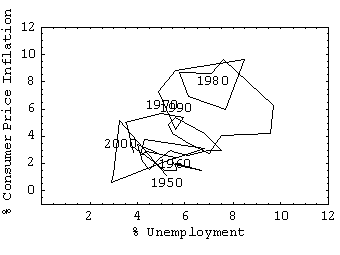
Figure 3. The unemployment - inflation space 1950-2001, Holland

Figure 4. The Netherlands, ‘official unemployment’ (drawn) and ‘not working’ (dashed)

Above rough division in decades suggests, as said, some ‘trade-off’. There is a discussion among economists whether such a ‘trade-off’ really exists, and in particular for the short run, but, with this division in decades, it cannot be denied that there are some systematic choices involved. Our object of study, stagflation, can be rephrased by observing that the Phillipscurve apparently has shifted to a higher and unfavourable position.

The authors Okun (1981), Hebden (1983), Blanchard & Fischer (1989), Friedman (1991), Phelps (1994) help to put the Phillipscurve in perspective. Extensive empirical work has been done by the Central Planning Bureau (1992a&b).

Okun (1981) emphasises the stability of the US Phillipscurve over the 1954-1969 period, but accepts that wages and prices thereafter are less flexible in the short run, due to ‘implicit contracts’ and ‘invisible handshakes’. Referring to Friedman and Phelps he notes: “In the sense that all economists must recognize that adverse shift of the short-run Phillips curve, they have all become accelerationists now (to reverse Friedman’s celebrated concession to Keynes).” (p239). Rather than getting lost in finding proper functional formats, Okun concentrates on formulating various elements that are important for policy making, indicating that a whole range of instruments must be used. The minimum wage gets short mention, but is not considered in relation to the Phillipscurve.

Hebden (1983) gives a recommendable review of econometric issues and empirical work (till that time) on the Phillipscurve, including (a) the original article by Phillips, (b) papers that remain close to his format, and (c) papers that include trade union influence and price expectations. Hebden notes:

“Models that seek to explain the causes of the inflation that has been experienced in the recent past, and hold out the possibility of helping economists to predict and maybe control inflation in the future, are sought after eagerly by economists and politicians. Many models have been produced and a fair degree of unanimity has been found as to the mechanics of the relatively mild inflation experienced in Britain in the 1950s and 1960s. But when inflation accelerated, in this country as in most of the industralised world, in the mid-1970s, those models were unable to cope; and though almost a decade of ‘hyperinflation’ has passed since then, no model that adequately explains its causes has yet been found.” (p158)

Blanchard & Fischer (1989) note:

“The Keynesian framework, embodied in the “neoclassical synthesis”, which dominated the field until the mid-1970s, is in theoretical crisis, searching for microfoundations; no new theory has emerged to dominate the field, and the time is one of explorations in several directions with the unity of the field apparent mainly in the set of questions being studied.” (p27).

On the Phillipscurve they note:

“The contemporaneous correlation between innovations in wage inflation and GNP is, however, positive and significant: it is this correlation that underlies the Phillips curve, which plays a central role in theories of the business cycle that allow aggregate demand disturbances to affect output.” (p19). [39]

Their discussion is critical and enlightening, but does not involve the role of the minimum wage. On p551 they discuss the high European unemployment, but then refer to the Layard & Nickell 1986 & 1987 model, concluding, a bit non-committingly:

“The Layard-Nickell model provides an example of how to relate the theories developed in this book to the data. It suggests a complex set of causes for high unemployment in which both demand and supply factors play a role and the labor market’s own dynamics explain the persistence of high unemployment with nearly stable inflation.” (p555).

Our analysis will allow a stronger conclusion. From the 1950s till the beginning of the 1990s the common view among economists and policy makers tended to be that the unemployment in the trade-off was “general” unemployment. This is not quite true for all economists, but many made this simplifying assumption. Nowadays we tend to link unemployment to lowly productive labour. For us it may be obvious, but compared to the earlier view of many it is a change of perspective that the once-thought-to-be “general” unemployment now turns up as a rather specific type. To make this change specific: we will hold that the unemployment in the trade-off has always been related to the distribution of productivity across labour.

Structure of the argument

The crucial insight is that the people who can demand pay rises need not be the people who run the risk of unemployment thereof. High productivity workers run less risk of unemployment and can more easily demand pay rises, while low productivity workers run the larger risk of unemployment. High productivity workers are more versatile and are able to shift the risk of unemployment to the lower income groups. When jobs are scarce, the high productivity workers even crowd out others from the labour market. [40]

The policy rule on taxes is: don’t tax low productivity labour. Why ? To keep it employed so that more productive labour will meet more competition and will not demand inflationary pay rises. In Europe, taxes on low productive labour are still high, causing a high minimum wage that causes unemployment. These taxes could be abolished, and without costs, since these workers are unemployed anyway. Similarly, marginal tax rates are less a problem than often said. The proposed alternative policy provides an improvement on both unemployment and inflation, exactly the kind of policy measure required for in the current situation.

This analysis is not common knowledge. It is missing in the economic journals, it is missing for example in Borjas’s (1996) much used textbook for undergraduates. Borjas (1996:441) states: “The minimum wage, however, affects mainly less-skilled young workers, so it is difficult to attribute much of the unemployment problem to minimum wage legislation.” [41] For policy makers, the OECD (1998) reports: “The cross-country evidence suggests that the minimum wage has no significant impact on overall adult employment.” though OECD (2000) is more guarded, see chapter 44. We will show however that a minimum wage can have huge ‘multipliers’.

The difference that it means

It is useful to clarify the difference between currect macro-economic policy in Western nations and what macro-economic policy can be according to this book.

Current macro-economic policy:

· accepts unemployment as a consequence of low inflation and reduced deficits

· sees the likely cause of unemployment in technology, globalisation and labour market inflexibility

· focusses on aggregates and averages

· discusses the distribution of wages mainly in terms of income (in-) equality.

The new macro-economic policy:

· sees a way to combine low inflation and balanced budgets with full employment

· sees the cause of current unemployment in the system of taxation

· focuses on distributions

· discusses the distribution of wages in its relation to productivity and unemployment.

Table 2 tabulates the differences.

Table 2: Differences between current and possible policy

	Current policy	Possible policy
low inflation & low deficit	accepts unemployment	full employment
cause of unemployment	technology, globalisation and labour market inflexibility	system of taxation
method	aggregates & averages	distributions
distribution of wages	income equality	productivity & unemployment

The new analysis means that we get a different perspective on the existing models.

For example, a current argument in Holland on labour market inflexibilities is that the replacement rate is too low. There would be a so-called poverty trap. People in a benefit situation would have little incentives to accept a job offer, since they would earn hardly more. This is regarded as a supply issue, and since one cannot raise wages (which would increase unemployment), the only solution seems to be the reduction of benefits. This was actually the statement of the Dutch Minister of Social Affairs at the presentation of the Dutch National Budget in September 1999. Even the small Socialist Party (SP) accepts this view, vide its January 2000 internet site. The Minister and the oppostion party however are misguided and badly advised. In the proper analysis the problem is crucially different. If there would be sufficient jobs then there already are regulations that people can be fined for not accepting a job offer. This fine creates an incentive of 30% in a warning stage and eventually 100% by full withdrawal of the benefit. So the problem is rather that there are insufficient job offers - with sounds more like a demand problem. By manipulating taxes, it is possible to reduce gross wage costs - and increase demand - while still allowing for a decent net income.

Another point of attention is the word ‘unemployment’. Holland in 1999 features an ‘official unemployment rate’ of about 3.2 %. It seems as if unemployment is no problem for Holland. As an economist I however cannot accept the sausage that the Statistical Office (in this case the Dutch CPB and CBS) here present. (1) Dutch ‘official disability’ is about 10% of the true labour force, (2) people older than 55 years are often excluded from the ‘official labour force’ too, (3) many people work part-time since they cannot find a full-time job, (4) many women will not work outdoors since childcare is too expensive because of the wrong wages, (5) etcetera. Many economists classify these issues under the denominator of ‘participation’, and then agree that Holland has a participation problem. However, in proper economic terms it is unemployment: people who would want jobs but cannot find them. I urge the statisticians to remain servient to economic science, as they claim they are, rather than servient to politics and disinformation.

13. Unemployment via taxes and minimum wage

Let us see in stylized fashion how it went wrong in 1950-2005. Our discussion uses Holland as the example to clarify the general OECD situation. The discussion will also use simplifying assumptions and few footnotes, to keep the text transparant. These defects will be remedied in the subsequent chapters.

Key aspects are:

· heterogeneous labour, and the use of an earnings distribution

· the minimum wage and unemployment

· decomposition of the minimum wage in subsistence and tax burden

· analysis of the Tax Void

· differential indexation

· dynamic marginal tax rates

· consequences for the macro model: spillover and domino effects.

Figure 5: Earnings distribution

The earnings distribution

Figure 5 gives an earnings distribution of a standard lognormal shape. The figure approximates the situation in Holland 2002, though without parttimers. With each level of income there is a number of ‘personsyears’ of people who earn that level. The earnings distribution can be used to compute how large unemployment will be below the minimum wage. Figure 6 gives the situation for the Dutch minimum wage of about € 18.3 thousand. Since Dutch unemployment is about 25% of a potential labour force of 8 million people, the graph conforms to the facts. [42]

Figure 6: Unemployment below the minimum wage

Analysing the minimum wage

We wonder how the minimum wage comes about. We see two terms in the minimum wage, as can be seen in equation (13.1a) and its explanation:

M = minimum wage [43]

B = subsistence [44]

T = arbitrary tax function

Bentham = Bentham tax function [45]

y = an arbitrary level of income

r = marginal rate

x = exemption

(13.1a) M = B + T[M]

(13.1b) Bentham[y] = r (y - x) for y > x,

= 0 for y x

(13.1c) Net[y] = y - T[y]

The minimum wage provides subsistence and thus consists of that net minimum and the taxes at that minimum, which is expressed by (13.1a). Since net income must be larger than B, this means for the Bentham function:

y - r (y - x) B & equality at M M = (B - r x) / (1 - r)

Malthus has subsistence B enforced by nature. Under current rules of (European) welfare states, B can be higher, since people who cannot earn subsistence B are entitled to a benefit of that level. [46] Table 3 gives the Dutch example.

Table 3: Tax wedge at subsistence (single person)

Dutch legal minimum wage 2002 (per annum)	€
Gross minimum wage in the official statute	15,638
Net, after deduction of taxes incl. premiums for the employee (single person)	12,516
Gross minimum wage: gross + premiums for the employer	18,265
All taxes incl. premiums (though exclusive of VAT etc.)	5,749
Tax as a percentage of gross minimum wage	31.5 %
Tax as a percentage of net income	45.9 %

The Dutch situation is depicted in Figure 7, the tax plot. The horizontal axis gives income y, the vertical axis the tax t. The tax line T[y] gives the Dutch tax brackets. Net income is given by the difference between the tax and the 45-degrees line (t = y). Subsistence causes the line y - B parallel to the 45-degrees line. This line cuts off a part of net income. The intersection of the subsistence and tax lines gives y - B = T[y], and this solves into the minimum wage y = M. You must earn at least M to satisfy the minimum net income requirement B.

Figure 7: Tax plot

Figure 8 clarifies that the minimum wage means that there are no full time wage earners below M, so that tax and net income are only relevant above it.

Figure 8: Tax plot revisited

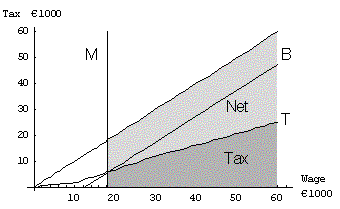
Figure 9 gives gives the same result but then as a net income plot. The horizontal axis gives income, the vertical axis net income. The tax is given by the difference between net income and the 45-degrees line. Subsistence now is a horizontal line at B. The intersection of the B-line and the net income line gives the minimum wage M. You must earn at least M to satisfy the minimum net income requirement B.

Figure 9: Net income plot

The Tax Void

Let us now combine the earnings distribution and the tax plot.

Note that the tax figures have shaded areas only above the minimum wage. The tax appears effective at and above the minimum wage, but not below it. Though taxes are defined below the minimum wage, there are no taxes collected, since people are unemployed below the minimum wage. The clear area from net minimum till the gross minimum wage M can be called the Tax Void.

The difference between net and gross is called the tax wedge, and it is generally seen as a vertical jump. There is a change of perspective now, in that we see it also as a range, particularly relevant for the minimum wage.

In the Tax Void the tax code has only a paper function (in terms of tax collection). The tax code helps to drive up the minimum wage, but it does not collect any revenue. Abolishing taxes in this area therefor does not cost anything too. Note that abolishing the tax void would mean that exemption would be chosen at subsistence.

Figure 10: Tax Void Unemployment

Part of unemployment below the minimum wage is still above subsistence. If taxes would be abolished in that section, then the affected people could still earn a living wage, and need no income support. This kind of unemployment can be called the Tax Void Unemployment. Figure 10 gives a plot of that section (shaded) for Holland.

For the record: the Dutch minimum wage only holds for fulltimers, and not for parttimers. Holland has a lot of parttime work (for that reason). We have eliminated parttimers from the present analysis.

Cause of the Tax Void

How has the tax void come about ? Since abolishing the tax void does not cost anything, and would generate a lot of employment, why don’t we abolish it ? Why do we continue the present absurd situation of mass unemployment ?

It appears that the situation has come about gradually, by a mechanism that is difficult to observe directly. It involves the co-ordination of tax policy with social policy, specifically the indexation of taxes and subsistence.

First note that OECD countries adjust their taxes for inflation, see OECD (1986). Tax exemption in 2002 will often be close to the inflation-adjusted real value of 1950. On the other hand, research in social psychology shows that subsistence tends to rise with the general level of income, the growth of which consists of inflation and real growth (or real net income). So there is “differential indexation”. In the 1950s exemption was pretty close to subsistence, so that there was no void to speak of. Since then, exemption has lagged behind the standard of living. When tax exemption lags behind net subsistence, then there is a multiplier effect on gross subsistence, with an accelerated increase of the tax void. This process also explains the ‘squeezing of income differentials’ in OECD countries.

Holland is the example again. In 1951, exemption for a single person household was € 354 and for a couple without childern € 463. At that time there was no official minimum wage, but it can be taken at that value. The price level in 2002 (1951=1) is 6.25 and the wage index 2002 is 25.59. This allows us to construct Table 4.

Table 4: Development of tax exemption in Holland

Euro’s	1951	1997	2002
Inflation index (%)	100	545	625
Wage index (%)	100	2082	2559
Exemption, single person	354	3223	8025
Idem, price adjusted	354	1930	2211
Idem, wage adjusted	354	7369	9060
Exemption, couple without children	463	6445	*13116
Idem, price adjusted	463	2524	2892
Idem, wage adjusted	463	9638	11850

* Dutch readers can find the computation in Colignatus & Hulst (2003)

Till 1997, official exemption € 3223 lagged strongly behind the wage adjusted 1951 value € 7369. In recent years the gap has been reduced, but the 2002 official exemption of € 8025 still lags more than € 1000 behind the wage adjusted 1951 value. Most important, it lags € 4500 behind the (single person) net minimum wage of € 12500.

Taxes

If we index tax parameters on inflation only, then this affects exemption x in the Bentham tax function, and thus x should be included in the function call.

P = price index

x[0] = exemption at the
base year

xi = real exemption index

(13.2a) x = x[0] xi P (and here xi = 1)

(13.1b’) Bentham[y, x]

(13.2b) Bentham[y, x[0] P] = r (y - x[0] P)

We also write the tax function as T[y, x] and net income as Net[y, x].

Subsistence

The indexation of subsistence differs from other incomes. When wages follow, on average, an index wi, the real subsistence index rsi commonly follows the net average wage, i.e. the wage after taxes.

W = the average wage (nominal)

W[0] = the average wage in
the base year

wi = wage index = W / W[0]

rwi = real wage index = wi / P

B[0] = subsistence in the base year

h = B[0] / W[0]

rsi = real subsistence index

rnai = real net average wage index

(13.3a) W = W[0] wi = W[0] rwi P

(13.3b) Subsistence = B = B[0] rsi P

(13.3c) rsi = rnai =
Net[W] / P / Net[W[0]]

(13.3d)

Deduction of the real net average income index

We choose the base year so that x[0] = B[0]. Let W[0] be the average wage in the base year, and let h = B[0] / W[0] be the base year ratio with subsistence. Then the index of real (net) subsistence rsi is set to the index of the real net average wage rnai, and is (proving (13.3d)):

with B[0] = W[0] h:

(13.3d)

For example, if base subsistence is half the base year average wage, B[0] = ½ W[0] then h =0.5. When r = 0.5 then rsi = 0.33 + 0.67 rwi.

With h and B[0] given, the causal chain is {rwi, r} rsi B M u. [47]

When all incomes grow as fast

Before we continue it is useful, however, to first clarify a formal property for the Bentham tax function.

Property (13.3e): For the Bentham tax function: There is equal growth of gross and net income, if and only if exemption is indexed on either.

Note: The distinction between (13.3d) and (13.3e) is that the former indexes x[0] on P only, and the latter indexes x[0] and B[0] on wi = P rwi.

Corrollary: Under (13.3e): If the income distribution remains the same (all incomes grow with the same rate) then also the average income, y = W grows at the same rate, and then also the net income distribution remains the same, and then the ratio of net average to subsistence remains the same too. Note: Western nations thus could wisely index subsistence and exemption on gross average income.

Note: These relations seem obvious enough, but actually proving it turned out to be a bit tedious.

Proof: Denote y[+1] = (1+gr) y = g y for growth rate gr, and Net[y[+1]] = n Net[y] (both g and n one period indices).

Net income with the Bentham tax is Net[y[+1]] = g y - r (g y - X) with X the new exemption. This should be equal to n Net[y] = n (y - r (y - x)). Thus n is defined by:

g y - r (g y - X) = n (y - r (y - x))

() Take z = g = n. Then z y - r z y + r X = z (y - r y + r x) and this gives X = z x.

( g) Take X = g x. Then g y - r(g y - g x)) = n (y - r (y - x)), so that n = g.

( n) Take X = n x. Then

g y - r(g y - n x)) = n (y - r (y - x))

g y - r g y + r n x = n y - n r y + n r x

g y - r g y = n y - n r y

g (1 - r) y = n (1 - r) y

g = n

Q.E.D.

Development of the Tax Void

These formulas call for a graphical illustration. We only need data on rwi, r and h for a stylized display. We will take r = h = 50%. Then we need data on rwi, and we can use our example of Holland.

Graphical presentation of the Dutch data

Appendix Table 20 gives the required data on the Dutch economy. Dutch 1951 exemption can be taken as 1951 subsistence. Before we use the data for the formula, let us first see what they mean. Figure 11 and Figure 12 on inflation P and real income growth rwi = wi / P show that the data fit above classification of subperiods for inflation and real income growth behaviour.

Figure 11: Continued inflation, stagnating real wage

Holland, 1951 = 1

Figure 12: Inflation plotted against the real wage

Holland, 1951 = 1

Using the data for our analysis

We now use the data for our analysis. There are four combinations of gross/net and real/nominal. This results into Figure 13. ‘Subsistence’ is always measured as a net term, and ‘minimum wage’ as a gross term. For Holland, we find that real subsistence has risen about 4-fold since 1951, and the nominal minimum wage more than 30-fold. The computed nominal minimum wage relates well to the factual 2002 minimum wage. Not only inflation accounts for the rise, but also an increased tax burden (that encounters inflation again).

Figure 13: Different indices at the minimum [48]

Holland, 1951 = 1

It was the slow rise of subsistence B and the lagging of exemption x in the 1950-1975 period that caused a multiplied rise of M, creating the Tax Void. Also, since the earnings distribution is nonlinear (lognormal), there was an even sharper nonlinear increase in unemployment.

Figure 13 shows that the real values stagnate since about 1980, and that the development since then is determined by inflation. Since inflation does not occur in the rsi index, the real situation is stable. For example, the gross-to-net ratio at the minimum since 1980 is quite constant.

Note too that this in a sense presents a difficulty. The problem with the minimum wage was caused before 1980, and policy makers wanting a solution in 2002 will rather look at the last decennium rather than to the 1950-1975 period.

Marginal tax rate & VAT

While the above considers exemption x, the analysis can be extended with an analysis on the marginal tax rate r.

Many economists hold that a high marginal tax rate is a disincentive for labour effort. They frequently propose a change from the income tax to the Value Added Tax (VAT). If we assume the same total tax revenue then the VAT might allow for a lower marginal tax rate, for the reason that the VAT has no exemption. At least, that is commonly conjectured.

Above analysis already exposes one flaw to the argument ‘in favor of the VAT’. Having no exemption means a higher minimum wage ! So, those tax theorists who propose a shift from income tax to VAT tend to neglect an important part of labour market economics. Note that a higher VAT on luxuy cars does not affect the subsistence worker who cannot afford these, and hence there is some truth in the statement that a VAT sometimes can be preferred. However, once we have solved unemployment by proper labour market policies, the discussion about income tax or VAT could be done in terms of fiscal properties only, and it might quickly appear that a low VAT of say 5% suffices. [49]

Secondly, it is said that a VAT taxes profits too and thus seems to allow a general reduction of the price of labour. But it raises costs disproportionally for the lowly productive (who generally work with less capital).

Figure 14 shows the development of the relative revenue shares of Dutch income tax and VAT for a selection of years (i.e. 1975, 1980, 1985, 1990, 1997 and 2003). The Dutch minimum wage problem has worsened also by this development.

Figure 14: Revenue shares of income tax and VAT

Marginal tax rate & dynamics

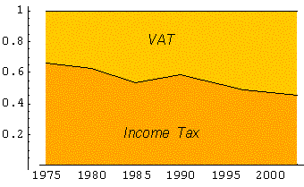
I agree with the basic idea about the disincentive effects of marginal tax rates. Namely, economic theory assumes maximising agents, and the condition for a maximum can normally be expressed in terms of marginals. However, the marginal must be computed correctly. Above marginal rate r is only a static rate, that applies to a specific regime, for example a specific period. However, tax rates are adjusted from year to year. A dynamic situation requires a dynamic analysis.

Let y = y - y[-1]. Then the proper (dynamic) marginal tax rate is DMR = T / y. For the Bentham function:

Generally the dynamic marginal is lower than the static marginal. In fact, when tax parameters are indexed in a certain way, then the tax can have the same growth rate as income, and then the dynamic marginal rate equals the average tax rate. This holds for individuals and for the macro data if all individuals are on a balanced growth path. Let the balanced growth rate be bgr:

(13.4)

The following is a small example of how a dynamic marginal rate can equal a normal average. Let exemption be $10000, and let the statutory marginal rate thereafter be 50%. Someone earning $50000 pays the tax of $20000, on average 40%. Let all incomes grow 5%, and exemption be indexed on national income. Then exemption becomes $10500, income $52500, tax $21000, again 40%. Thus on the (dynamic) “marginal dollar” this person doesn’t pay 50% but 40%.

For the Bentham tax function we can derive a simple expression for individual growth. We are most interested in expected developments. Let personal income grow by rate , so that y[+1] = (1 + ) y, and let exemption be expected to be adjusted by rate , so that x[+1] = (1 + ) x. Then we find:

Let us regard the dynamic marginal rate for a Dutchman in 2002 who considers an increase in work effort for 2003 (and beyond), and let us assume a regime of sound economics. In the ideal case, exemption in the base year is put at subsistence, in this case € 12.5 thousand. Ideally, subsistence rises with income, and not just real net average incomes. This ideal implies that exemption is adjusted not just for inflation, but for the nominal growth of income. Let us assume this ideal, and let us assume that national nominal growth is 4%, for example consisting of 2% inflation and 2% real growth. Let us then regard the situation of a single economic agent. He knows that next year exemption will be adjusted with 4%. He has to judge whether it is worthwhile to him to invest or to increase labour effort, so that his income will rise. If his personal income rises with 4%, then his dynamic marginal will be equal to his present average tax rate. If his personal income rises by 8%, then his dynamic marginal will differ; it will depend upon his actual income level, but anyway will be less than the statutory marginal rate of 50%. Figure 15 gives the plot of the dynamic marginal for those two rates, for various levels of income. The 4% line here also gives the average tax level.

Figure 15: The dynamic marginal rate

Individual income grows at 4% or 8%, while national income grows at 4%
and the statutory marginal rate is 50%

Empirical analysis often shows marginal rates to be less relevant - and average tax rates to be more important - than ‘common theory’ claims. This analysis on the dynamic marginal provides a useful part of the explanation.

Spillover and domino effects

Above analysis concerns minimum wage unemployment. The next question is how this relates to other kinds of unemployment.

It is useful to observe that the analysis in these pages is new. Concepts like the tax void, differential indexation and dynamic marginal tax rates, and the insights on their interaction, are really new, and have been concocted by me in a search for new scientific results. That means that governments have not incorporated these concepts in their policy making (even though the occasional civil servant may have been aware of some phenomena). Policy making up to now has been based upon a different analysis, and, alas, by being different from the right analysis, the governmental analysis is a wrong one. This is not without consequence. By analogy, when a patient gets a medicine based on a wrong diagnosis then the illness may get worse rather than diminish. In the present case, the tax void unemployment has important spillover or domino effects on unemployment above the minimum wage, and the channel of transmission is the misguided policy reaction up to now.

For example, in the 1970s governments tried to stimulate the economy by incurring big deficits, but they ended up with inflation. In the 1980s and 1990s governments opt for low inflation, and they end up with high real rates of interests and mass unemployment in Europe and poverty in the United States.

For example, Dutch economic policy is based on a general restraint on wages. This policy has fueled Dutch exports and reduced Dutch imports. The general restraint in fact subsidises exports, and Holland runs an external surplus for quite some years now. The internal imbalance is reflected in an external imbalance. The proper policy reaction however would be a wage cost policy targetted at the minimum.

Diagnosis and Therapy

Please note that the present review only gives a diagnosis, and that it is a different affair to find the proper therapy. The first is necessary step before the second can be considered.

In the course of some years I have experienced that discussing therapy is useless when people do not even understand the diagnosis. Policy makers tend to be focussed on therapy - but judge this from a wrong diagnosis. For example, in The Hague in 1992 (at a social-democratic political rally when I was no longer a member of his party) mr. Wim Kok, the Dutch Prime Minister of 2000, occasional chairman of the European Union and the social-democratic ‘respected elder’ to mr.-s Clinton, Blair, Schröder and Jospin, and a person who did some basic econometrics in his younger years, laughed loudly when I suggested to raise Dutch tax exemption from the then € 3 thousand to € 10 thousand. He must have thought of staggering costs, and it didn’t help when I said that it need not cost anything.

A major remark about therapy is that to undo the damage of the last four decades, it is not necessary to take four new decades. Return to optimality can be much faster.

The alternative and new policy would be to abolish taxes in the tax void and to allow people to earn their own - decent and untaxed - living. This alternative policy reminds of an old rule. The Dutch economist Cohen Stuart proposed in 1889 (cited in Hofstra (1975)) to put tax exemption at the level of subsistence. To drive the point home he drafted the following analogy:

“A bridge must carry its own weight before it can carry a load.”

In 2005 there is the additional argument that abolishing void taxes will not cost anything, while nations will save benefit payments due to more employment.

Note that the ideas of Cohen Stuart’s ‘bridge’ and the tax void are not very complex in themselves. In 1991 I explained them to a 12 year old kid and he commented: “A child can understand that.” Still, the EU and its score of modern governments sin against these concepts.

If unemployment is inefficient, then by definition there is a Pareto optimising solution, that will not cost anything. Most economists don’t believe in cheap solutions. Much of the debate hence focusses on ‘efficient unemployment’, where the sad state is caused for example by globalisation, technology or ‘welfare state scelerosis’ (with poverty traps). But, clearly, the tax void exists, it is a cheap way out, and the other arguments will turn out to be ghosts, which they already can be shown to be.

Note though that some period of transition may be required. Policy makers will be hesitant, advisedly, about an overhaul of the tax system. Note, then, that the tax system defines our notion of a subsidy. A wrongly levied tax, in this case the tax void, can be compensated for by a wage cost subsidy. [50] Abolishing the tax void is more sensible in the long run, but since this can only be done gradually, then some general subsidy directed at lowly productive jobs would speed up short term adjustment. The rule would be that those subsidies are reduced when tax exemption rises towards subsistence.

Stagflation resolved

More employment.... Does that not fuel inflation ? The pieces of the puzzle fall into their places when the tax void is related to the unemployment & inflation problem. The steady rise of the tax void explains the track record of unemployment and inflation. The 1950s have been characterized by relatively low taxes on low income earners, and this allowed for full employment and low inflation. From the 1960s onwards the lagging tax exemption started causing problems with unemployment. The tax policy since at least 1965 enhanced the imbalance of the internal bargaining positions of labour instead of counter-balancing it. Hence inflation was persistent, and high levels of unemployment were required to achieve price stability.

As said, governments suffer from a co-ordination problem. How governments reacted in the past depended upon the view of the day. Since the proper solution was not known, the problem did not go away. The differential indexation of tax exemption and the social minimum did not draw attention to itself. Each year adds only a slight effect which is hard to see. But over the years the void has accumulated, and with huge consequences. And the problem will remain with us in the future unless policy changes.

The co-ordination problem persists, currently. Governments currently regard minimum wage unemployment as just one type of unemployment, and not even the most important type. Current policy is based upon other explanations for unemployment, notably those of technology, globalisation and flexibility. The policy reaction based on these views is to reduce taxes for higher incomes, so that they are encouraged to work, invest and spend more, and so that labour market flexibility might be increased. However, the ineffectiveness of current policy can be explained by the fact that these views are not entirely logical. The arguments of technology, globalisation and flexibility run up against contradictions:

· Technology is a source of wealth, and it boosts the productivity of the lowly productive jobs, making the problem of poverty and unemployment less serious than it would otherwise have been.

· “Globalisation” is a scare word for “trade”. Trade however is another source of wealth, and it too has been with us for ages. Rising wealth in distant countries means rising wages over there, and trade itself thus puts limits to foreign competition. Japan over the last 60 years is a prime example of this phenomenon, but every rich nation has had the same experience.

· The “flexibility” or “welfare state sclerosis” argument can only explain that the US has poverty and Europe unemployment, but it does not explain that there is a problem with low productivity jobs in the first place. The poverty trap as said does not exist.

Thus to be sure: the real policy target is low inflation, and policy makers only discuss technology, globalisation and sclerosis/flexibility in a second line of the argument. This second line is essentially a cop-out, since it does not concern the real issue - and a discussion can be very tiring if people behave like that.

At the same time, the wrong policies work counterproductively. The reduction of taxes for the higher incomes obviously is financed by a reduction of provisions for the lower incomes, aggravating the minimum wage and poverty problems.

In my analysis, the present situation bears another surprise. We diagnose current unemployment as inefficient. Be sure that you see what inefficiency means: it means that there is a solution that is beneficial to some and that does not hurt others. Having a bright idea always means a “win-win” situation or a free lunch. In the present case there is the move to full employment under price stability. The present unemployed will find jobs. The higher productivity group will have a theoretically larger risk of unemployment, but in practice this risk will be modest as in the 1950s. The real gain for the higher income earners will come from the services that will be provided by the jobs of the presently unemployed. So you do not need to reduce taxes for the higher paid, since they already will have a real gain at current income.

This was it, in a nutshell. Now I beg your understanding. My analysis is more complex than can be stated in these few lines. Both tax policy and social policy are quite complex themselves, and this certainly holds for their interaction with inflation and unemployment. For example, you may ask why I haven’t discussed income redistribution effects. Actually, this is because the alternative policy could be neutral to the income distribution. The reason for this is that the analysis focusses only on the link between wage costs and productivity. But you might want to hear more about this. Also, you might ask whether above explanation covers all possible cases of unemployment and inflation. Of course it doesn’t. The analysis does help to clarify that other types of unemployment need other types of policy, such as education and so on. But you might want to hear more on that too. These are just examples of issues, and there are many more issues that need to be dealt with. Which space forbids. However, given that my model amends existing economic models, much of the required explaining is ‘existing economics’.

This novel explanation is in the tradition of Keynes and Tinbergen while it fits in with mainstream economics. When economists check and confirm these findings, our economies are likely to enjoy more growth with full employment and low inflation.

14. The 1974 Duisenberg disaster

While the above uses a stylized example of Holland, there is a short and enlightening story about actual Dutch politics, far remote from econometric regressions. Quotes are here in my translation, Dutch readers can also read Colignatus (1994b:28).

In Dutch politics, parties have to form coalitions to be able to govern, and the Biesheuvel 1971 cabinet came about by a coalition agreement that contained the following plan:

“Increase of tax exemption (in the direction of equality exemption for married couples with one child towards the minimum wage (….))”

The explanation of this idea to parliament was (MvT 1971/72):

“(…) it doesn’t require more adstruction that current exemption is too low. Its size doesn’t satisfy the fundamental notion of a threshold, the exemption of taxation of part of income, that is reasonably required for financing the necessary means of existence as seen in contemporary social views.”

This plan didn’t succeed, the government broke down prematurely. There came about a new leftist government under leadership of Den Uyl, and his Minister of Finance was Wim Duisenberg, the president of the European Central Bank in 2000. This cabinet however rejected above concept. The 1974 argument was:

“De government (…) explained that the social minimum had been raised in the preceding years in such extent that it could be considered to provide means to pay taxes.”

The latter statement is rather shocking. Subsistence is by definition a net concept, and the politicians don’t stick to that definition. The statement also means that someone who falls in the tax void is forced into a benefit situation. [51]

What is alarming too, is that Duisenberg was not alarmed, didn’t veto this nonsense.

After this ‘Duisenberg disaster’, the issue disappeared from people’s mind, it got transformed into an annual debate on indexation and the topic of discussion became the level of benefits for the needy. In 2005 Holland still suffers the consequences.

Book IV
Presentations for the general public

In March / April 1996 I put two presentations for the general public in the Economics Working Papers archive at the Washington University at St. Louis. In August 1998 there was a third paper. [52] These papers are directed to a general audience, and to teachers and students. Since this current book basically addresses economists and uses quantitative methods, I doubted whether I should include these texts here, also since there is some overlap that can be distracting. There however are two good arguments to include them with little adaptation: (i) Once a fellow economist is starting to grow convinced of the value of my analysis, then he or she will face the same problem of explaining it to others. These texts then can be of use. (ii) The historical date of these texts underlines the co-ordination problem. Even when a good summary was available, and even when the moral imperative facing Western nations was clearly formulated, our failing systems of economic policy making limped along, and caused misery upon misery for many of its citizens.

15. Unemployment solved !

A breakthrough in economic theory

Since the early 1970s Western economies have been plagued by mass unemployment and the threat of inflation. Over the years since then various economists have proposed various possible solutions, but never quite convincing ones. Now there is a novel analysis that means a breakthrough in economic theory. The present author is quite certain that the “missing link in the model” has been found. If true, this analysis offers guidelines for full employment under price stability, just as Western economies enjoyed in the 1950s. The main point is: don’t tax lowly productive labour. Why ? To keep it competitive so that more productive labour will not demand inflationary pay rises. Though this new analysis is only in the stage of presentation and introduction at the scientific fora, there is no reason to withhold the present rough sketch for a general public.

It is well-recognised these years that Western economies have a problem with jobs with a low level of productivity and thus a low level of market-earned income. The United States tolerate more poverty - the working poor - while Europe sets its minimum wage much higher so that Europa has more unemployment.

This problem with low productivity jobs finds various explanations, notably those of technology, globalisation, and inflexibility - the latter ornate for “welfare state sclerosis”. Policies based on these latter explanations have been enacted for some time now. For quite some time, in fact; while little is being achieved. It is proper that we pose the question: why is it that we don’t achieve much ?

Unemployment obviously has a much longer history than the current problem. Also, the Western track record on unemployment can only be understood when the record on inflation is taken into account too. Economic science has much to say on the complex relationship between inflation and unemployment. Now, we are forced to be brief here. We will concentrate on what is new and on why it is new.

We set out with the empirical evidence since 1950. This track record can be divided in meaningful decades:

· The 1950s had low unemployment and low inflation.

· The 1960s had the threat of unemployment, and governments accommodating inflation in order to actually prevent it.

· The 1970s nevertheless had mass unemployment bursting into the open, and governments accommodating high and accelerating inflation to battle it.

· The 1980s-till-now had governments come down hard on inflation, and accepting high levels of unemployment as the price for stability.

One sees a certain “trade-off” between unemployment and inflation. From the 1950s till the end of the 1980s the common view among economists and policy makers was that the unemployment in the trade-off was “general” unemployment. Nowadays we tend to link unemployment to lowly productive labour. For us it may be obvious, but compared to the earlier view it is revolutionary that the once-thought-to-be “general” unemployment now turns up as a rather specific type. To make the revolution specific: we will hold that the unemployment in the trade-off has always been related to the distribution of productivity across labour.

Now obviously, when this is new, then it has not been recognised before, and then it has likely been missing in policy. And policy that was based on a wrong analysis, is likely to have been the cause of the very problem that it wanted to solve.

Let us see how it went wrong. Regard the legal minimum wage and note that people are not allowed to work below that minimum. Note too that there hence will be no earnings that can be taxed in that range. We can call this range the “tax void” or “tax vacuum”. However, tax statutes are defined in that range anyhow. Tax statutes in that void are actually used to define the gross minimum wage. In Europe, the high gross wage will cause unemployment and its related benefit burden. In the US, the void is reduced a bit by accepting poverty. In common economic terms: tax policy and social-economic policy are badly co-ordinated.

How this has come about is a story of a more technical nature. First note that OECD countries adjust their taxes for inflation. Tax exemption in 1996 will often be close to the inflation-adjusted real value of 1950. On the other hand, research in social psychology shows that subsistence tends to rise with the general level of income, the growth of which consists of inflation and real growth. So there is “differential indexation”. In the 1950s exemption was pretty close to subsistence, so that there was no void to speak of. Since then, exemption has lagged behind the standard of living. The inflation-adjusted subsistence of 1950 may be only a third of 1996 subsistence. When tax exemption lags behind net subsistence, then there is a multiplier effect on gross subsistence, with a fast increase of the tax void.

The alternative and new policy would be to scratch taxes in that void and to allow people to earn their own - decent and untaxed - living. This alternative policy reminds of an old rule. The Dutch economist Cohen Stuart proposed in 1889 to put tax exemption at the level of subsistence. To drive the point home he drafted the following analogy: “A bridge must carry its own weight before it can carry a load.” In 1996 there is the additional argument that abolishing void taxes will not cost anything, and that nations will save benefit payments due to more employment.

More employment.... Does that not fuel inflation ? The pieces of the puzzle fall into their places when the tax void is related to the unemployment & inflation problem. The steady rise of the void explains the track record of unemployment and inflation. The 1950s have been characterized by relatively low taxes on low income earners, and this allowed for full employment and low inflation. From the 1960s onwards the lagging tax exemption started causing problems with unemployment. The tax policy since at least 1965 enhanced the imbalance of the internal bargaining positions of labour instead of counter-balancing it. Hence inflation was persistent, and high levels of unemployment were required to achieve price stability.

How governments reacted depended upon the view of the day. Since the proper solution was not known, the problem did not go away. The differential indexation of tax exemption and the social minimum did not draw attention to itself. Each year adds only a slight gap which is hard to see. But over the years the gap has accumulated, and with huge consequences. And the problem will remain with us in the future unless policy changes.

Current policy is based upon other explanations. Notably those of technology, globalisation and flexibility. The ineffectiveness of current policy can be explained by the fact that these views are not entirely logical. The arguments of technology, globalisation and flexibility run up against contradictions. Technology is a source of wealth, and it boosts the productivity of the lowly productive jobs, making the problem of poverty and unemployment less serious than it would otherwise have been. “Globalisation” is a scare word for “trade”. Trade however is another source of wealth, and it too has been with us for ages. Rising wealth in distant countries means rising wages over there, and trade itself thus puts limits to foreign competition. Japan over the last 40 years is a prime example of this phenomenon, but every rich nation has had the same experience. Finally the “flexibility” or “welfare state sclerosis” argument can only explain that the US has poverty and Europe unemployment, but it does not explain that there is a problem with low productivity jobs in the first place.

The present situation bears another surprise. We diagnose current unemployment as inefficient. Be sure that you see what inefficiency means: it means that there is a solution that is beneficial to some and that does not hurt others. Having a bright idea always means a “win-win” situation or a free lunch. In this case it is the move to full employment under price stability. The present unemployed will find jobs. The higher productivity group will have a theoretically larger risk of unemployment, but in practice this risk will be modest as in the 1950s. Their real gain will come from the services that will be provided by the jobs of the present unemployed.

Policy makers will be hesitant about an overhaul of the tax system. Note, then, that the tax system defines our notion of a subsidy. A wrongly levied tax, in this case the tax void, can be compensated for by a wage cost subsidy. Abolishing the tax void is more sensible in the long run, but when this can only be done gradually, then some general subsidy directed at lowly productive jobs would speed up short term adjustment. If only those subsidies are reduced when tax exemption rises towards subsistence.

This was it, in a nutshell. Now I beg your understanding. My analysis is more complex than can be stated in these few lines. Both tax policy and social policy are quite complex themselves, and this certainly holds for their interaction with inflation and unemployment. For example, you may ask why I haven’t discussed income redistribution effects. Actually, this is because the alternative policy could be neutral to the income distribution. The reason for this is that the analysis focusses only on the link between wage costs and productivity. But you might want to hear more about this. Also, you might ask whether above explanation covers all possible cases of unemployment and inflation. Of course it doesn’t. The analysis does help to clarify that other types of unemployment need other types of policy, such as education and so on. But you might want to hear more on that too. These are just examples of issues, and there are many more issues that need to be dealt with. Which space forbids. However, given that my model amends existing economic models, much of the required explaining is ‘common economics’.

There remains one major point. That tax exemption is low, is defended by OECD governments with the argument that it keeps marginal rates down. And the attractiveness of low marginal rates is that they spur economic activity. My finding however is that the latter claim is only true when the marginal rate has been defined properly. Thus I agree with the claim, but it must concern the proper marginal tax rate. There is a difference between the proper rate, which is dynamic, and the rate used by OECD governments, which is the static and statutory rate. Dynamic analysis shows that the proper marginal rate will be close to the average rate. This part of my analysis is important for economic growth. Having less unemployment will mean lower average taxes, and thus lower proper marginal rates, and thus more incentives for sustainable growth. For many of my fellow economists it is this part of my analysis that will come as the greatest surprise of all. However, this is not an issue that can be settled in this review, and here I definitively have to refer to my extensive analysis.

This novel explanation is in the tradition of Keynes and Tinbergen while it fits in with mainstream economics. When my fellow economist check and confirm these findings, our economies are likely to enter into a new high growth path with full employment and low inflation.

Allow me to add the personal note that I am overjoyed by these findings.

(March 1996)

16. Enable Russia to help itself

World developments in the 1990s show a worrysome parallel to the 1930s with the Great Depression. Present-day Russia reminds of the pre-war Weimar republic, where a devastated economy and weak democracy allowed Hitler to take power. Western nations in the 1990s hinder trade with Russia and the Eastern nations for fear of unemployment at home, as they did in the 1930s with Germany. If trade were stimulated instead of hindered, Russia could regain economic and political stability by itself. The moral problem is not external and does not concern whether Russia would need financial aid. The moral problem is internal, and concerns whether Western political leaders are willing to face their own errors that cause the present mass unemployment at home.

Russia is shrouded in a veil of doom. A nation once proud about its achievements, is now, as so many feel, humiliated in the face of history. A loss of empire, a collapse of economic security, some coup attempts in both Kremlin and Duma, a rising reign of violence by a mafia in the main cities and by full-blown fighting at the geographical fringes, and a political arena that smells more of fear than of confidence. Like the Weimar republic in pre-war Germany, Russia has been subjected to the rules of chaos, and yet again the odds are risky - and risky for the world at large.

Something needs to be done. Something smart, something humane, something effective and efficient, and something courageous. Therefor, something which is not likely to happen quickly. However, there is one single possibility that is very much worth of our attention. It is something what we actually could do. And what - given the risks of this moment - we should do

It is trade that will help Russia and the Eastern nations to recapture economic security and thereby regain political stability. And, since it is our fear of unemployment that motivates us to block that trade, Western nations should tackle unemployment at home directly.

Parallel

Our comparison of present-day Russia with pre-war Germany is no coincidence. World developments in the 1990s show a worrysome parallel to the 1930s. The 1930s suffered from the Great Depression. In the 1990s the world is again plagued by mass unemployment. Again there is a major region that is economically devastated and that desperately needs access to the world market, and yet again the other wealthier nations hinder that entry, while concentrating shortsightedly on their own problems at home, and neglecting the consequences of neglect. The West might want to reduce the risk of a Russian disaster, but not at the cost of jobs at home. Trade barriers are there to keep cheap Eastern products from “flooding” its home market. Europe throws in huge subsidies for its agricultural exports. Western tariffs or quality requirements are pitted against Eastern exchange rates, in a war on trade whatever its consequences on economic and political stability.

The West is dugging in and seems to repress the recognition that history is repeating itself. Again the world finds itself in a deadlock, and yet again chaos feeds on it.

But we should remember the trade war of the 1930s and the rise to power of Adolf Hitler ! In the 1930s the same mechanism of trade, unemployment and political instability applied. In this period it was Germany that was the weak nation. The Versailles Treaty of 1919 that ended World War I put Germany under a huge reparations bill. The world forgot that the war had been started by an autocratic Kaiser and that Germany now had a new, fidging democracy. To pay that bill, this weak democracy was obliged to cut imports and to spur exports. The reparations bill worked like a foreign tariff that took away funds that could have been invested otherwise. By the end of the 1920s Germany defaulted on its international debt - and thereby indirectly caused the Wall Street Crash of 1929. Thereafter, all nations scrambled for the life-boats. Nations feared for their home markets and employment, and defended themselves by exchange rates and tariffs. In their fear they made things only worse. The German economy collapsed, and on the teutonic waves of resentment its weak democracy toppled and Hitler took power.

Let us now compare: Is the Russian democracy anything other than new and fidging ? Have its generals not tried to seize power ? Have its tanks not roared against its very own Parliament building ? Has its economy not dropped by a third? Or conversely, have all its nuclear weapons and uranium stores been savely secured ? Have the Western nations done their utmost in opening their markets ?

Risk not chance

Of course, there is a glimmer of hope. The Russian capacity for suffering is impressive. Few nations could sustain this suffering and national disgrace without lapsing into resentment, cruelty and violence on a much larger scale than we actually see in Russia. The West has provided some funds and done something more. The world is not at war and may not be at war for some time. The probability that things go right is large, and there is only a small chance that things go wrong.

But please consider: If the only glimmer of hope is that the world is not at war, then the situation is quite depressing. Hope is not the point, and neither likelihood nor expectation. The point is risk. Risk comes from the arithmetic of loss multiplied by chance. Thus: risk = loss * chance. If things go wrong in Russia then the consequences will be huge, and a small chance times a huge loss gives a risk too large.

Internal not external

The West should open its eyes and see the economic logic. Eastern nations need to take part in the international economy and thus need modern Western equipment. To buy the latter goods they need the proper currency. Either someone gives them that foreign currency, the dollars, yen or marks, or they have to earn it themselves by exporting. To simply give them credit, on the scale required, is absurd. Therefor it is access to Western markets that is essential for those nations and for political stability. Indeed, if they had access, and if the flow of trade were to start, then the World Bank and IMF could extend credits and thereby fuel the process towards stability.

At the same time, economic science tells us that it is not trade that has caused present Western unemployment. Marking trade down as the culprit, and using trade barriers to solve a situation that trade has not caused, only makes things worse.

The moral problem is internal and not external. The cause of present-day unemployment in Western economies is internal management and not external trade. There is a failure within the internal co-ordination of macro-economic policy, a failure by our very own governments. Western nations could tackle their unemployment problem at home - if only our political leaders were willing to take a hard look at their own internal policies.

The historic parallel also concerns the current lack of attention for the internal question. Policy makers that concentrate on an external trade war neglect the internal opportunities. There is the following sobering story about the economist John Maynard Keynes. From the early 1930s Keynes advanced his solutions to the Great Depression, and this culminated in his 1936 book that changed macro-economics. Policymakers could have reacted already in the early 1930s, ... but only did so after World War II had already begun.

Conclusion

We might ask: Do we care about the peoples of Russia and the Eastern nations ? And should we act with economic sense ? However, those questions are imprecise. The real question is whether our leaders care so much that they will reschedule their busy agenda’s and really look into a problem that they cause themselves.

There is every reason to believe that political leaders are quite deaf on this. So pray that there will not be a new world war. So shout to your political leaders: Stop that trade war !

Do something about external trade tariffs and internal unemployment. Enable Russia to help itself.

(March 1996)

17. Will the West repeat Versailles ?

Asia and the Eastern European nations are in a state of economic turmoil. An important element for improvement is that Western nations open their markets to more trade. This is in fact what the West could have done after the fall of the Berlin Wall. But petty shortsightedness of the governing elites in the West blocks this kind of solution. The situation reminds one of the Versailles peace conference after World War I that fostered a lot of resentment and helped cause World War II. The basis conclusion is that sound economic advice is not listened to. The best advice on how to steer out of the current world macro-economic mess is that every parliament installs a committee to enquire into the process of economic advice. They could study the books by Paul Krugman, and possibly also my analysis on unemployment and my suggestion for an Economic Supreme Court.

Western nations show an inadequate reaction towards the Eastern nations since the fall of the Berlin Wall, and this inadequate reaction is repeated with respect to the current economic throes of Asia. The West displays disinterest in the hardship and actual physical pain inflicted on millions of our fellow human beings, and a neglect of the long run effects of this egotistic behaviour. Part of this inadequate reaction however is also caused by wrong applications of economic theory, so that true compassion that is out there doesn’t get the chance to show itself. One lesson is that Western nations are advised to restructure their policy making process so that governments are better served with proper economic advice.

The negligent way that the Western nations treat the other nations reminds one of the Versailles peace conference after World War I. Historians agree about the sad Western attitude at the Versailles conference. The Western Allies humilated Germany and subjected that country to decennia of economic hardship, purposely crippling its economy. These events caused a huge resentment in Germany, and this fostered the rise of Adolf Hitler. Also, Germany’s defaults on its financial obligations were a major cause for the 1929 Crash and the subsequent Great Depression. This episode is another example that two wrongs don’t necessarily make a right, and it also shows how wrongs can backlash at the wrong-do-er.

The lesson of Versailles is that opponents can often best be allowed to grow into a relationship of companionship and economic competition and co-operation for the betterment of all. Rather than subdue them or take advantage of temporary weaknesses, they could be helped so that they could help us. This lesson should now be applied to the current situations of Asia and Russia.

It is useful to recall that Western nations were not without proper advice at the time of Versailles. They were warned, and by nobody less than J.M. Keynes. As Paul Krugman recently stated about Keynes: “After that war he became famous as the author of The Economic Consequences of the Peace, an eloquent condemnation of the vindictive terms imposed on the defeated Germans; his concern was vindicated by the rise of Adolf Hitler, and the memory of his warnings helped convince a victorious America to aid, not punish, its prostrate enemies after World War II.”

Indeed, after World War II the Allies helped Germany and Japan to reorganise their countries and to prosper again. While the average citizen may be deluded by sentiments of nationalism, religion or ideology, it normally is a governing elite that abuses those sentiments for purposes of its own grandeur - and once a decent government is in place, there often appears little reason to blame that average citizen for the errors of its country. In the same way post-communist Russia deserves our sympathy, and the same holds for Asia with its different history.

But why has the West forgotten this valuable lesson ? Why do Western governments neglect Nobel Prize winner Jan Tinbergen’s work on the Optimal Economic Order, and why do we again have a show of petty egotism and shortsightedness ?

The reason is that the West is not immune to the same ‘governing elite’ processes that can be at the detriment of common welfare. The governing elites and bureacracies in the West have agenda’s of their own, and though they are restrained by democratic rules, these rules are not as strong as they could be. Our systems of checks and balances are a product of history, and not necessarily of the quality required. Politicians and bureaucrats often still can lie and get away with it. The United States e.g. had David Stockman on the budget deficit, and it took too long before that matter was settled. In general, sound economic advice still is obstructed by political processes, and policies and the electorate itself then grow misguided in their choices.

To better understand the failure of Western democracies on the issue of economic advice, one can best start by reading Paul Krugman’s books “The Age of Diminished Expectations” (1990), “Peddling prosperity” (1994), “Pop Internationalism” (1996), and “The accidental theorist” (1997). For example, when Krugman discusses US majority leader Armey’s book “The Freedom Revolution”, he states: “Armey is no fool. He cannot be unaware that he is fudging his numbers. Possibly he regards a small fib as justifiable in the service of a higher truth. Or possibly he has managed to achieve a state of doublethink, in which the distinction between what is politically convenient to believe and the objective facts no longer exists [sic]. The end result is the same: His book is an effort to obscure the stark realities (…)” (1997:60). Similarly, one can read in the American Economic Review that the US Council of Economic Advisers is rather proud of its achievements in the last decades, but we should be aware that this council is a bureaucratic body, and it hasn’t the independent position that could have protected the US economy from the events and errors as are related by Krugman in his “Peddling prosperty” saga or shown by the record of mass unemployment.

Let us now regard what the West could have done with regards to Russia after the fall of the Berlin Wall and the first free elections there - and what could be done now also with respect to Asia. I take my own 1996 paper “Enable Russia to help itself”, and quote from its summary: “Western nations in the 1990s hinder trade with Russia and the Eastern nations for fear of unemployment at home, as they did in the 1930s with Germany. If trade were stimulated instead of hindered, Russia could regain economic and political stability by itself. The moral problem is not external and does not concern whether Russia would need financial aid. The moral problem is internal, and concerns whether Western political leaders are willing to face their own errors that cause the present mass unemployment at home.”

Clearly, with this being the state of affairs, one can imagine the strength of the forces that prevent a proper discussion of these issues. Western companies embrace tariff barriers to cheap imports - and raise their own prices. Bureaucrats embrace barriers since these give a sense of control, and these also justify the very existence of this bureaucracy. Labour unions will fight unemployment at home with whatever misguided argument it takes. Governments embrace economic tales about ‘globalisation’ and ‘competition from cheap labour countries’ since these distract attention from home grown errors, and these goverments neglect economists who tell them that ‘globalisation’ and ‘competition from cheap labour countries’ are rather like fairy tales indeed. Krugman again uses the term ‘globaloney’ - and have you heard your President or Prime Minister adopting that critical attitude too ?

The best economic advice for the current situation is as follows - and I urge upon my fellow economists to adopt and spread that advice too: Every parliament could install a committee that will enquire into the process of economic advice. This committee could study Krugman’s books and my suggestions for a solution of mass unemployment and for an Economic Surpreme Court amendment to the national constitution(s). Nothing less will do. Note, by the way, that when countries start installing these committees, the markets will be quick to anticipate the directions of their conclusions, and economic recovery would already set in.

We all know Lincoln’s words: “You can fool all of the people some of the time, and you can fool some of the people all of the time, but you cannot fool all of the people all of the time.” Let us act upon it, or show Lincoln wrong. (August 1998)

Notes in 1999: (1) A 1999 UNDP report describes the Eastern European situation as disastrous, and calls for a quick joining up to the EU (De Volkskrant October 16 1999). It is courageous that an international body speaks up like this - and it indicates the seriousness of the situation. (2) The journalist Peter Michielsen in NRC-Handelsblad October 30 1999 rightly calls attention to the original borders between the empires of Rome and Byzantium. The Eastern European countries that are doing relatively well belong to the Roman area, the others to Byzantium. He mentions that this cultural distinction has also been noted by Andreas Oplatka of the Neue Zürcher Zeitung 1994, who again refers to George Kennan in 1945. I was a bit surprised by this, hadn’t thought about it in this way. (3) These points however nicely fit what I have been argueing for ten years now. Enabling people to help themselves starts with taking account of the local conditions; and overall the barriers to trade should go.

Book V
Methodology: Definition & Reality

18. How to check ?

At the Dutch Central Planning Bureau, I helped making the Athena model (CPB (1990)) with its 7000 variables. I had this model at my computer and could let it do tricks like an obedient dog. But a proposal to an exercise effectively like the above was rejected by the directorate, and nowadays I am no longer in the position to make such proposals. The desktop computer that I have now, in 2004, might have more power than the 1990 mainframe, but I don’t have the data, the programs, and the possibility of discussion with colleagues. I have Word for Windows, Mathematica, some crucial books, an occasional visit to the Dutch Royal Library, and the internet (at low speed). Moreover, I have to make a living, in a different kind of job, and my time constraints thus are severe. This explains why I am forced to a logical argument - and this explains again why I emphasise logic anyhow.

Thus, crucially: it is up to the fellow economists to check my findings. They / you should actually do this anyhow, since a critical perspective always is best. For example: What are the data on the minimum wages in the other OECD countries ? OK, the OECD internet site shows that 1997 statutory minimum wage is 39% of median wages incl. overtime in the USA, 60% in France, 30% in Japan, etcetera, quite sizable [53] - but what about the tax void, the development, the indexation, the discouraged workers below the minimum, etcetera ? [54] What about the shifts of the Phillipscurves in this light ? What about the effects of the dynamic marginal rate ? How are these topics in all nations ? And what would happen, if all nations gain confidence about growth policies again, and they fire up each other and move all to a new higher growth path ? Clearly, the research agenda is huge.

The situation since 1989-1991 has been a bit like this: Me stating that unemployment has been solved (analytically) and inviting the fellow colleagues to check it - and nothing further happening. This book should make a difference in that I collect the various articles that I have been able to write since then. When others see the whole route then they will also better see the crucial junction where to take the other turn.

This may also concern the novel contribution to methodology below. [55]

19. Dealing economically with concepts

Maximising information power

Methodology may be seen as ‘economics applied to science’. The methodology of economics is the fixed point in that construct - even economic methodology in the traditional form as presented by Tintner (1968).

The ‘basic economic problem in science’ is - in my perception or definition - that some set of concepts can better deal with the data than another set. New ideas are like manna from the sky, but the manna must be collected, stored, compared to the older findings, etcetera, and an optimum must be found, using scarce resources over alternative ends. This ‘basic economic problem in science’ thus is quite different from the ‘mundane (non-basic) economics’ that, say, 5% more truth can be traded against 10% more effort and cost.

The mind has the economic problem of dealing effectively and efficiently with (i) old concepts, (ii) new information and (iii) the construction of new concepts. The name of the game is to have concepts or definitions fit reality as usefully as possible. The definitions must be chosen as strong as possible, so that uncertainty can be shifted to observation (and the problems with observation).

The human mind seems to be occupied with reduction of cognitive dissonance - or, at least, that is a fruitful way to look at that mind. Here I follow Aronson (1992a&b), who provides a definition of cognitive dissonance, and data and tests that lend empirical support for it. It appears that a commonly used method of reduction of cognitive dissonance consists of the rejection of new information to the advantage of older views. Frequently the messenger is blamed for the bad message, and even, after the messenger has been punished, the bad news is neglected since it came from an unreliable source - namely a person who had to be punished (while it is forgotten that, if the news is considered irrelevant, then there was no base for punishment). Man is a rather prejudiced creature, and thus not so effective and efficient at information handling - but man has to handle new information.

Barrow (1998:4) [56] provides us with a useful quote:

“This unifying inclination of ours is a by-product of an important aspect of our intelligence. Indeed, it is one of the defining characteristics of our level of self-reflective intelligence. It allows us to organize knowledge into categories: to know vast numbers of thing by knowing rules and laws which apply in an infinite number of circumstances. We do not need to remember what the sum of every possible pair of numbers is: we need know only the principle of addition. The ability to seek and find common factors behind superficially dissimilar things is a prerequisite for memory and for learning from experience (rather than merely by experience). (…)

All human experience is associated with some form of editing of the full account of reality (‘we cannot bear too much reality’). Our senses prune the amount of information on offer. Our eyes are sensitive to a very narrow range of frequencies of light, our ears to a particular domain of sound levels and frequencies. If we gathered every last quantum of information about the world that impinged upon our senses they would be overwhelmed. Scarce genetic resources would be lopsidedly concentrated in information-gatherers at the expense of organs which could exploit a smaller quantity of information in order to escape from predators or to prey on sources of food. Complete environmental information would be like having a one-to-one scale map. For a map to be useful it must encapsulate and summarize the most important aspects of the terrain: it must compress information into abbreviated forms. Brains must be able to perform these abbreviations. This also requires an environment that is simple enough and displays enough order, to make this encapsulation possible over some dimensions of time and space.

Our minds do not merely gather information; they edit it and seek particular types of correlation. They have become efficient at extracting patterns in collections of information. When a pattern is recognized it enables the whole picture to be replaced by a briefer summary form which can be retrieved when required. These inclinations are helpful to us and expand our mental powers. We can retrieve the partial picture at other times and in different circumstances, imagine variations to it, extrapolate it, or just forget it. Often, great scientific achievements will be examples of one extraordinary individual’s ability to reduce a complex mass of information to a single pattern. Nor does this inclination to abbreviate stop at the door of the laboratory. Beyond the scientific realm we might understand our penchant for religious and mystical explanations of experience as another application of this faculty for editing reality down fo a few single principles which make it seem under control. All this gives rise to dichotomies. Our greatest scientific achievements spring from the most insightful and elegant reductions of the superficial complexities of Nature to reveal their underlying simplicities, while our greatest blunders often arise from the oversimplification of aspects of reality that subsequently prove to be far more complex than we realized.”

This human property should be used in economics to explain actual events. Colignatus (1996d) for example applies Aronson’s findings in social psychology to economics, trying to indicate the actual ‘forces’. Another application is the very analysis in this book, for example where we stated earlier:

“If the government on the one hand would desire to use the results of scientific advice for its budget process, and on the other hand would not opt for an Economic Supreme Court, then its definitions would be logically inconsistent, and it would thereby tend to create a cause for dishonesty and improper manoeuvreing and thereby corrupt its processes.” (above)

While the above relies on structural models, the property can also be modeled in the reduced form. Chapter 40 uses information indicator I {0, 1}.

Another application is to the methodology of science. Methodology should harness this human property, and clarify when it is useful and when it is misleading.

Science aspires at a more unbiased approach. This unbiased approach also means the deliberate creation of cognitive dissonance, by creating new concepts and by looking hard at the evidence till it doesn’t go away anymore.

The evolution of knowledge can be described in terms of an ever increasing power in the concepts used.

The introduction of a new definition is not simple. The questions always are: does the definition cover the facts as we know them, does the definition not introduce hidden aspects that cause confusion and prevent advancement ? If a new definition wins out, it is, apparently, only so because it is believed to have passed the test. Though, we should be critical of this assumption. Only if the environment is ‘critical’, then we might presume a ‘survival of the fittest’ for concepts. (And all this is reminiscent of Dawkins’s ‘memes’.)

Definitions can be devious in quite vulgar ways. In the English economics literature, ‘perfect competition’ is defined as the situation when no agent can affect the price, i.e. all agents are price takers. The Dutch word for this case is ‘full competition’. The English definition forces English economists to use the word ‘imperfection’ for all other cases. Even quite reasonable cases, in the normal state of human life, when agents have market power but balance at some social optimum, would be ‘imperfect’. Also a natural monopoly would be an imperfection - even if one could not conceive the situation differently since the monopoly is a natural one. It would be better if the English economists would adopt the Dutch definition, so that the words ‘perfect’ and ‘imperfect’ could be used in their proper sense depending upon circumstance. This is just a vulgar example of how definitions can lead one astray.

The competition of alternative concepts can be quite sophisticated however. Let us illustrate this with three examples. The most illuminating example may well be Pythagoras’s theorem and its relation to the circle. This problem concerns mathematics, so that the discussion is less taxed by semantics and empirical matters - though there is of course the theory about empirical space. The second example of ‘falsification’ is surely in the realm of empirics. The third example concerns the distinction between determinism and volition.

Pythagoras and the circle

Regard a triangle with perpendicular sides a and b and hypotenuse c. There are two points of view:

1. Pythagoras proved [57] that the square of the hypotenuse equals the sum of squares of the perpendicular sides, i.e. that a² + b² = c²

2. For the circle, it is taken as the defining quality of the circle, and thus accepted without proof, that the points are at equal distances from the origin. In other words, a circle with radius c is defined as the collection of points (a, b) at a distance of c from the center. Thus a² + b² = c² by definition.

The two points of view are presented in Figure 16. The definition of the circle can be taken for granted, since it is just a definition. On the other hand, it will be very useful to discuss the proof of the Pythagoras theorem, since then we see the need for a proof.

Let us take the square with sides z = a + b and surface z * z = z² = (a + b)². Within this square we can see four triangles with straight sides a and b and hypotenuse c, as has been done in Figure 16 in the square on the left.

In the square, another tilted square has been drawn, with sides c and thus a surface of c². There are four surrounding triangles, each triangle has a surface of ½ a*b. The surface of the large square is equal to the surface of the tilted square and the four triangles.

Figure 16: Pythagoras and the circle

Thus:

· From the big square itself: z² = (a + b)²

· From the tilted square and the triangles: z²= c² + 4 ab/2.

Elimination of z then gives a² + b² = c².

This proof has been taken from DeLong (1971), and he remarks that Pythagoras proved it differently.

How do we explain that one and the same equation can have two interpretations that are so widely different, one with the need for complicated proof and the other with direct acceptance by definition ?

There may be other explanations, but I think the following will do fine. Note that the definition of the circle relies on the notion of ‘distance’. There are two points of view again, so that point 2 above actually splits in two parts:

2A) Basically the (Euclidian) distance between two points can be measured by a straight line section. That is rather simple, and makes for a readily acceptable definition of a circle.

2B) However, in a system of co-ordinates, that distance can be reinterpreted in a representation in terms of the co-ordinates. There are two possibilities again. Either the distance can be defined as simply the formula dist[{x, y}, {a, b}] ((x - a)² + (y - b)² ) with {x, y} the origin - above {x, y} = {0, 0} - or it can be defined geometrically as the hypotenuse of the differences of the co-ordinates. If either definition is accepted, then one can use Pythagoras’s theorem to derive the other.

The essential difference between (2A) and (2B) is that (2A) is elementary and poor in concepts and results, while (2B) is complexer and rich in concepts and results. Viewpoint (2A) only allows us to use measuring rods between arbitrary points and little else. We are allowed to sweep the rod around the center, and thereby draw the circle, but then it somehow stops. Viewpoint (2B) allows us to do much more. A line between two points is interpreted in terms of a system of co-ordinates, and that opens the scope for new results.

We find that the opposition of (1) against (2) is rather messy, and (2) actually hides two suppositions. The ease of (2) depends directly upon the ease of (2A), while (1) actually compares with (2B) that is complexer. The phrase “In other words” in (2) above thus was misleading, and actually represents the introduction of another assumption.

With this clarified, we also note that (2) is stronger than (1), and that it was possible to seduce the human mind to accept (2) rather easily. There has been a progression in concepts, resulting in stronger definitions.

Note that behind all this there is a notion of empirical space. In (1) there is a hidden assumption of a flat space. In (2B) the assumption is made explicit, and then open to amendments (curved surfaces, or abstract spaces). The movement of (1) to (2) thus is, partly, (a) the advancement in concepts by means of the definition of distance (and the circle as a collection of equal distance points), (b) the introduction of the separate step of observation - with the difficulties: when does the definition apply to reality, or if there is some reality, how do I select the proper definition ?

The point that is relevant for this book then is: that the definition is so good, that it in practice substitutes for many everyday empirical problems. A criterion for a good definition is: that it can be such a substitute.

When a definition is a close substitute for reality, then it may percolate into common culture with more authority. For example: every citizen can establish the existence of a tax void and Pareto suboptiomal unemployment purely from the logic of the level of gross minimum wages and the official tax statutes - and we don’t need big computers or official bureaus to do some econometrics and then tell us.

Admittedly, there is danger in seductive and seemingly right but wrong definitions. If ‘child’ is defined as ‘irresponsible young human’, then we may be tempted to treat children as such and forget to expect the responsibility that they can handle. But the existence of this danger should not make us close our eyes to the advantages of good definitions.

A side issue concerns our concept of ‘space’. Let us first consider an example of cultural relativism. It appears that different human cultures can have different approaches to one’s orientation in space, and that these approaches are wired into the languages used. [58] Taking a point of reference can be done in three ways: (1) Relative: taking one-self (“the tree is to the left of the house” - seen by me); (2) Absolute: taking the sun (“the tree is to the west of the house”); (3) Intrinsic: taking one of the objects (“the tree is to the back of the house”). If someone is asked to copy a situation in front of him towards a place in the back of him, then there will be a different ‘copy’ depending upon one’s language/culture. If you have a cup of coffee and a pencil in front of you, pick them up, turn yourself around, and recreate the scene, then a Westerner will use relative positions, while an Australian Aboriginal will use absolute positions (and turn the relative positions around). The question now is: while this only concerns the point of reference, can we imagine something similar that affects our concept of space itself ?

I take the position that the human mind apparently is able to conceptualise Euclidean space - and that this actually defines our concept of space. If we take a non-Euclidean geometry - such as a globe - then this still can be imagined to exist within Euclidean space. Pythagoras’s theorem is invalid for triangles drawn on a globe, but to hold that space is a globe would be erroneous - since our definition of space would be Euclidean.

One of the questions often posed is whether the universe - interstellar space - is Euclidean or not. This is a badly posed question. If we define space as Euclidean, then it is another question whether a ray of light follows a straight line or is deflected by gravity.

Barrow (1998:p42-44) provides a troubling quote: [59]

“The most important consequence of the success of Euclidean geometry was that it was believed to describe how the world was. It was neither an approximation nor a human construct. It was part of the absolute truth about things. (…) This confidence was suddenly undermined. Mathematicians discovered that Euclid’s geometry of flat surfaces was not the one and only logically consistent geometry. (…) None had the status of absolute truth. Each was appropriate for describing measurements on a different type of surface, which may or may not exist in reality. With this, the philosophical status of Euclidean geometry was undermined. It could no longer be exhibited as an example of our grasp of absolute truth. (…) These discoveries revealed the difference between mathematics and science.”

This quote is troubling for the following reasons:

1. If we define ‘space’ as Euclidean, then it is an absolute truth. This definition seems to maximise our information power. Other surfaces can be imagined within that space.

2. One might think of ‘empirical space’ as something that must be measured. The idea is: ‘If it cannot be measured, then it is not relevant.’ OK, this seems fine in principle. But if a physicist would use ‘light’ as a measuring rod, then this is asking for problems. Namely, Euclidean geometry already provides us with our system of measurement. Defining ‘empirical space’ differently would conflict with our original definitional grasp of space. Better is: to stick to the definition, and regard measurements that deviate - e.g. from gravitational deflection - as the physical properties of the objects and measurement tools involved.

3. That there is a difference between mathematics and science does not disqualify the notion of absolute truth. A true deductive sequence ‘Assumption Conclusion’ has absolute truth. And it should be realised that scientific theories are mathematical (with the scientist working on an assumption).

4. It is possible to translate the Dutch ‘lijn’ as ‘point’, and ‘punt’ as ‘line’ (thus conversely) and still find a consistent model for Euclid’s axioms. But this is a mathematical exercise, and it does not necessarily have to do with ‘space’.

So it seems that Barrow and I agree for 99%, but still, the 1% difference features big in some dimension. Note that the discussion here concerns more a side issue, but it remains useful to indicate the deeper aspects of Pythagoras’s theorem.

Falsification

The ‘principle of falsification’ is that hypotheses are only scientific if they are formulated such that they are vulnerable to empirical testing, and might be falsified. It has been formulated by Popper, see Keuzenkamp (1994).

The principle has two disadvantages: (1) purely logical, (2) stochastically.

(ad 1) Take logic first.

Counterargument 1. Regard the statement All ravens are black. This statement will be false when one finds a non-black, say white, raven. So the statement would be an acceptable scientific hypothesis, since falsification is possible in principle. But, as the falsificationist would hold, it would remain a hypothesis, and we should be aware of the fact that is only a hypothesis, until it had been checked for all ravens (Tintner (1968:12)). This falsificationist view however is problematic, since most of us will sense that there is truth in All ravens are black, for example by our definition of a raven.

Counterargument 2. In the extreme, all scientific knowledge would consist of instances of falsification. It has been falsified that the Earth is flat, that atoms cannot be broken, that ... But the principle itself, i.e. that ‘all scientific knowledge would consist of instances of falsification’, is a definition and is not open to falsification.

While falsification may be a successful research strategy in many cases, it does not seem to be a fully satisfactory way of organising science, at least from these two points of logic.

(ad 2) Take stochastics next. Let us regard the typical modelling situation:

The model:

Estimation:

Observation X[+1] forecasts:

Final observation:

y = X ß +

y = X b + e

y_est[+1] = X[+1] b + Exp[e[+1]]

y[+1]

The question now is whether this new observation can falsify the hypothesis of the empirical estimate. This question is not as simple as the naive falsificationist first had in mind. The principle of falsification is formulated as for deterministic reality, while many empirical models are stochastic. In stochastics, there may be deviations, and sometimes large ones. There are problems of measurement in y and X, the choice of the functional relationship, missing variables, and the choice of the stochastic specification itself.

One useful empirical answer is optimal control, with the example of a rocket launched to the moon, where there is continuous adjustment to observed error (‘falsification‘). This control only works well when there is a proper definition of the loss function. The issue of the loss function is a crucial one, but this is not falsificationism.

Logic and stochastics cause me to take the following position.

There is a difference between all₁ (universal) and all₂ (generally, usually, normally). The statement All ravens are black can be seen as:

1. a definition. It then holds universally. Empirical truth then is conditioned to the logical tautology of the definition that we have chosen. If we find a white bird that looks like a raven, it cannot be a raven. (But we think that this definition covers reality, for example since we have some ideas about genetics and evolution.)

2. an empirical statement - grounded in a stochastic model. It is shorthand for All ravenlike birds tend to be rather black or whatever the professional might deem correct. The meaning of such statements is more subject to context than in the case of well-groomed definitions.

The human mind thus faces the choice: To adopt a definition and run the risk that this does not fit reality so well, or to adopt a statement on averages and work out more details of the empirical loss function. Decisions on such statements thus are sensitive to the loss function, but the second category requires more detail.

This of course does not solve everything. The distinction of these two dimensions or perspectives is not like solving all problems in their domains. Also a definition like All ravens are black by definition does not answer the question whether a particular object is a raven or is black. Is a size of 10 kilometers acceptable ? Did we look in daytime or at night ? Must it be alive, and then, what is life ? So the distinction between definitions and empirical statements is useful, but it does not solve all problems. The point is not quite that one can always adjust definitions, but rather that a definition is not reality by itself. (Though it can get close.)

At one point in history, scientists were willing to accept the periodic system of elements to catalogue the wide variety of materials around us. There was apparently little loss involved in accepting these definitions, or Lavoisier’s periodic table was more gainful than other catalogs. The definitions did not change the materials, but facilitated more efficient research. At one point in history, see Mirowski (1989), economists were willing to analyse human behaviour in terms of utility maximisation. The approach is an empty box, since any behaviour can be described as such. For example satisficing behaviour can be represented as minimising the distance from satisfaction. Also in ‘evolutionary economics’ the utility maximisation model can be applied though these researchers are critical of this approach. (While, curiously, Charles Darwin was inspired, amongst others, by Adam Smith.) The new approach for laboratory experiments makes us even more critical about the rationality hypothesis. Utility maximisation however helps organising one’s thoughts, helps professional discussion, facilitates modelling and empirical estimation, and is generally considered an advance above less explicit approaches.

As with the Pythagoras example, but now empirically, there is a switch from just empirical knowledge to a set of definitions, when the loss function allows it.

Kuhn (1962) describes major changes as ‘paradigm switches’ (though someone noted that he used that word in perhaps 40 ways). I rather draw attention to the change from empirical knowledge to definition. This change need not be a paradigm switch. Paradigm switches may be the most intriguing or flashy examples of the introduction of new definitions, but the change from empirical knowledge to definition does also occur in ‘normal science’.

Determinism and free will

Holland around 1600 had the theological argument between Gomarus who defended predestination and Arminius who defended a measure of volition. This discussion had started before them, didn’t end with them, and continues till this day, also in these pages.

The 20^th century gave a novel twist to the argument, namely quantum mechanics. Instead of the folly of the gods, there now is a randomizer with a scientific garb. If objects, and the molecules in our brains, have random aspects, then this would be neither determinism nor volition. Quantum mechanics normally is applied at the micro level of particles, and there is the suggestion that larger aggregations of masses still would behave in the Newton-Einstein fashion. Schrödinger however gave an example - his cat - how quantum mechanics could also extend into this macro world. So the challenge to the debate on predestination is real. [60]

The quantum model is stochastic of itself. This differs from the randomness caused by simple measurement errors - the randomness commonly used in economics. However, economics has some purely stochastic models of itself too. There is for example the Erlang queueing model. Consider a postoffice with clients arriving and being served. Interarrival and service times can be modeled with exponential distributions, and this allows us to determine the average length of the queue, the average waiting time, the average utilisation rate of the service window, and such. If the situation gets more complicated, then research economists use computer simulation models to find the best way of operation. This example shows that economics already is familiar with a model that is stochastic in itself. Note that there are some ways to re-introduce a degree of determinism - as your barbershop may require you to make an appointment. The basic observation that we make here is that the stochastic approach is basically a modeling method, and there is no implication that arrival and service are intrinsically random.

The discussion above introduces the various components, and the question now becomes what to make of it all. The following gives my solution.

First of all, science by definition avoids the ‘deus ex machina’ assumption. An understanding of reality is looked for without reference to a god. So our discussion is not burdened with the associations of eternal damnation (and predestination to this).

Secondly, science by definition aspires at a deterministic understanding. Scientists may adopt a stochastic approach with only a limited degree of accuracy, but the target remains a 100% accuracy - which is determinism. Hence, by definition, scientists have a deterministic predisposition. [61] [62]

Thirdly, the idea of a ‘free will’ is a moral category, differing from physics. Admittedly, the scientific approach would presuppose that our moral considerations depend on our brain, and the movements of electrons and molecules that could be caught in a determistic model - but the proper conclusion is that we don’t have that model yet. The existence of time, and in particular the uncertain future, is a precondition for morality. An ‘existence proof for God’ would be that in the limit of time, prediction accuracy rises to 100% and all moral beings are going to make the proper moral choices. [63] But we don’t know for sure that those choices will be really moral - and anyway it is hard to see how this could affect us. For example, we may predict, as social scientists, that when economic conditions worsen, that politicians then may be more inclined to morally dubious choices. But we need the passing of time to determine whether this prediction materialises - and, as human beings, we would still want to form a moral opinion and discuss the moral aspects. The conceptual gap between ‘ought’ and ‘is’ remains. Eventually there might be a practical (non-conceptual) bridge, but for those same practical reasons it isn’t there yet.

Though science does not refer to gods, we can use a god anyway for clarification. Janus, the Roman god and name-giver to the month of January, had two faces, one to the past and one to the future. Figure 17 uses the Janus head as an analogy to locate the various concepts.

Figure 17: Janus head analogy

Note: This only displays the three opposing concepts in one picture,
without implying that all concepts to the left are equal
or that all concepts to the right are equal.

The Janus head analogy works only up to some degree. We don’t know all that happened in the past, we can use probability statements for the past too, and thus we cannot replace ‘past’ with ‘certainty’. Similarly, as said, science has a deterministic predisposition, so the future basically is predetermined from a scientific point of view. Yet the head analogy is useful, since it focusses our attention to these various subtleties.

Thus, clearly, the Arminius and Gomarus debate can be seen as non-sensical if they got the two categories of science and morality confused. Even though we can have a deterministic predisposition, we still can have moral volition (and be judged by jurors on making wrong choices). Their debate would be proper in so far as Gomarus would take predestination in a moral sense - but then the debate is not relevant for us.

Thus, clearly, quantum mechanics drops out as a fundamental category. It only remains as a research strategy in the face of apparent difficulties, but it still is on the road to 100% accuracy.

Admittedly, quantum mechanics itself seems to pose that nature would have random properties at the micro particle level. Some even argue that this would be the basic example of true probability - while all other ‘examples of probability’ (like throwing dice) are basically deterministic (and we only use probability techniques to make up for our lack of knowledge or laziness in measurement). In particular, Richard Gill, professor in mathematical statistics at Utrecht university, gives this argument at a roundtable discussion:

“We should be collectively ashamed not to know anything about quantum mechanics. I would like to see all introductory texts in probability theory going a little into the physical (quantum) theory behind the geiger counter before using some data of alpha particle counts as an illustration of the Poisson process; I would like a discussion of the Bell inequalities together with a modicum of quantum mechanical background to show how elegant probabilistic reasoning shows that the quantum world is truly random (unless you would like to go for an even more weird non-local deterministic theory).” (1997b)

Indeed, also economists are familiar with the concept of Brownian movement, or the random walk, and use this model for example in analysis of the stock markets. Or in the labour market, with labour supply LS and employment LE, unemployment is u = 1 - LE/LS: but u then basically is a probability, since the model does not provide an additional explanation why one person works and the other doesn’t.

But Gill’s argument does not convince me. The point is: you may pose that nature would be such, but you don’t know for sure. You are still using only a model. The scientific challenge remains to develop a model that increases accuracy.

Yes, there is the Heisenberg uncertainty model that if you measure position then you no longer know speed, and if you measure speed then you no longer know position: and this model nicely captures a basic notion of uncertainty. But, try for a better model then - and take some thousands years more to do so. [64] [65] [66]

As a corollary, we can take a position on path-dependency (hysteresis) and chaos.

Some authors use the word ‘chaos’ in the sense of path-dependency. For example, a small variation in first conditions (starting point, parameter) can cause a widely different result - a butterfly flapping a wing can cause a tropical storm. Since we already have the term ‘path-dependency’ for this, we better reserve ‘chaos’ for the meaning of ‘seemingly random’. A chaotic system, in this proper sense, then gives a fully deterministic description, but the outward appearance that some variables would be random. Here it is strange that people who are in favor of ‘chaotic modeling’ also use this to be against determinism.

Path-dependent and chaotic models can be useful. The orbit of Earth around the sun looks solid, but over the billion years it seems pretty random. There is Schrödinger’s cat model that shows the macro world depending upon a micro state. There are the strange models in history and biology, where for example a meteor wipes out dinosaurs. OK, all these models exist, and they can be real good descriptions of true states of nature. But all this does not disprove the definitory deterministic predisposition of science. If you would run the movie again from the start (which is currently said to be a Big Bang, but I don’t know about that), then you would get, by the models that science tries to develop, the same result. If you would argue that anything else might pop up, and your mother could be a dinosaur with a pig’s head, and if you would develop models that would show this, then you are quite in danger of being out of science. (You would drop out on this definition, but could be in on the other criteria.)

Concluding this section, we find that definitions indeed guide our understanding of nature. The definition of science itself guides our perceptions - for example when it guides us into taking quantum mechanics as a model only instead of as ‘reality itself’.

A reason to be strict about this definition of science is that people, who would argue that nature is basically random, would also tend to reject deterministic results of science. A deterministic result of science is for example (1) that divergent indexation of tax exemption and the standard of living causes a tax void, and (2) that the existence of a tax void can be used to ‘abolish taxes’ without costs. It would be a pity if this result were to be rejected because of a fundamentalist ‘random view of the world’.

From stylized fact to definition

Our subject is the political economy of western welfare states, and in particular employment and inflation aspects. This subject is quite complex, and we must be modest about our results. Of course we can use statistics of the national accounts, and thus indirectly we use the statistical labour of thousands of statisticians, and indirectly the results of thousands of firms and of millions of citizens that filled in their tax forms. Economic literature provides a wealth of models and interpretations of these data. In my case, I also rely on my own experience in constructing a national economic model. All this, however, does not mean that we can forget about modesty, on the contrary. Nevertheless, it is my conjecture that we can achieve a more enduring result than just awareness of complexity.

What is interesting in economic discourse is the concept of ‘stylized fact’. When an economist observes some regularity, he is rather inclined to use that term. We shall use the term more conservatively, and we are hesitant about observing regularities. But we also can fruitfully employ the term when there is a regularity indeed. In some cases, when the regularity is so strong that our loss function comes in the epsilon zone, then we even can switch to definitions.

So we adopt the methodology:

(a) state what we consider to be the stylized facts

(b) define our concepts so that the stylized facts are covered by definitions

(d) link back to conclusions about reality.

A proposition - as a statement on reality - can be regarded as a mathematical theorem about/within a model of stylized facts. When there is a tautology, we attain truth by definition.

We here deliberately refer to Bochenski (1956, 1970:20): “The word ‘proposition’ has been variously used, (...) nowadays commonly as the objective content of a meaningful sentence”.

Some students of the History of Economic Thought will see a clear resemblance of above methodology and what Schumpeter called the “Ricardian vice”. Quoted by Tintner (1968:7):

“His interest was in the clear-cut result of direct, practical significance. In order to get this he cut this general system to pieces, bundled up as large parts as possible, and put them in cold storage - so that as many things as possible could be frozen and “given”. He then piled one simplifying assumption upon another, until, having really settled everything by these assumptions, he was left with only a few aggregative variables between which, giving these assumptions, he set up simple, one-way relations so that, in the end, the desired results emerged almost as tautologies.”

This is almost exactly what we shall do, except that we generate tautologies.

Step (d) comes closest to the Popperian falsificationist criterion. Our deductions need not be insulated against testing, even though this present book abstains from econometric testing since we are too much involved in creating our concepts and constructing consistent and useful propositions. [67] Abolishing the Tax Void is a good and cheap test anyway for the relevance of this analysis.

It is useful to keep Solow’s comment in mind:

“There is something deeply satisfying - not to say suspicious - about any proposition that seems to deduce important assertions about the real world from abstract principles.” (1976:148)

So, advisedly, the reader better checks what we are doing here, and governments should run their own regressions and models before they make policy decisions. But of course I only dare to present my results here since I am confident that they, in the hands of competent and true scientists, allow a real advancement.

Relating to Hicks 1983

In his essay “A discipline not a science” (1983:365-375), John Hicks argues that economics is too far from the accuracy reached in the material sciences, and explains that he cannot ‘altogether’ deny that he himself has converged on a ‘critical’ attitude. This attitude concentrates on the clarification of terms, i.e. their definitions, also by using quite unrealistic models. For example: “Though the concepts of economics (most of the basic concepts) are taken from business practice, it is only when they have been clarified, and criticised, by theory, that they can be made into reliable means of communication.” (p372-3).

Hicks then concludes that economics is a Discipline. His quote of Keynes (in II.7) above is taken from these pages. My position on this is twofold - the position of hard science with soft data. On one hand I embrace the critical attitude. Indeed, we should develop sound definitions, and remain critical about how these are applied in communication. That is the meaning of the Definition & Reality methodology. And it brings us far, since we can advise to abolish the Tax Void without running regressions and a computer model. On the other hand, Tinbergen’s efforts have not been in vain, and models with estimated coefficients are useful tools for policy analysis. For example, some economists may reject the existence of a Phillipscurve, and all economists should be critical about the data and the parameter values, but such a relationship remains useful in a macromodel that is used for evaluation of policy alternatives. It would be curious to accept the concept of a ‘model’ and to accept other relationships like a consumption function, and reject the use of a Phillipscurve: even though the uncertainties are quite comparable.

In other words, our method remains econometrics, even though we end here with an increased awareness of the role of definitions. We are just in the phase that running regressions is useless if the model is no good. Regressions come in only when we have a good candidate, and regressions even might benefit from some definitory relationships. We even would like to do those regressions ourselves if we had the data and the time. So, for now, let us first develop what we conjecture to be the proper model.

20. Structural and reduced form

There is the useful distinction between the structural and reduced form:

· the structural form represents actual relations as good as possible,

· the reduced form gives the simplest representation, with the interaction minimised.

With y a vector of endogenous variables, x a vector of exogenous variables, and f and g functions, then a structural form is y = f(y, x) and a reduced form is y = g(x).

Since econometrics can only approximate reality, the true structural form can only be approximated. What we consider to be a structural form is an intersubjective consensus. We anyhow have to adopt an approximation, which means that many factors have been removed. However, for two models we can often clearly see that one is simpler than the other, and then we can usefully apply this distinction between the structural and reduced form.

The distinction between structural and reduced form also affects the structure of this book. The next chapters concern the structural form, actually starting with the textbook IS-LM model. We relax the assumption of homogeneous labour, and introduce heterogeneous labour. First we look at labour supply only. Then we look at supply and demand, and at the equilibrating dynamics, which causes the topic of the Phillipscurve. We show how the Phillipscurve and the Constant-Wage-Inflation Rate of Unemployment (CWIRU, a.k.a. NAIRU or natural rate) shift as a consequence of minimum wages or poverty. We then relate minimum wages and poverty to developments in taxation. The co-ordination failure on taxes and minimum wages not only causes the internal imbalance on the labour market, but also an external imbalance, with international trade.

The discussion of the structural form results into the need for more scientific clarity. Though much seems to depend upon empirical parameters, some aspects however are more fundamental. This leads to the discussion of the reduced form. We first develop a theorem on the influence of taxation on employment and unemployment regimes in welfare states. Since taxation depends upon social choice, we then discuss Arrow’s theorem on social choice (structural form again). We also note that there may be a confusion about inefficiency and the existence of a ‘free lunch’. Having established the possibility of rational social choice, we then develop a theorem on stagnation in the policy making process (reduced form again).

21. Direct application to the Economic Supreme Court

In chapter 8 we stated: “If the government on the one hand would desire to use the results of scientific advice for its budget process, and on the other hand would not opt for an Economic Supreme Court, then its definitions would be logically inconsistent, and it would thereby tend to create a cause for dishonesty and improper manoeuvreing and thereby corrupt its processes.”

We can directly apply our Definition & Reality methodology. The point is that desiring for a scientific base and not making a Court is logically inconsistent. Parliament and President may ‘define’ their ‘Council of Economic Advisers’ as ‘scientific’ but when there are little safeguards, then reality takes over, and the Council will de facto not have sufficient power to resist political meddling.

The appendices contain an example draft for a Constitutional Amendment for an Economic Supreme Court and a description, taken from the White House internet site, of the CEA. The difference should be clear.

Law-givers know: If a law does not fit logic and reality, then people will see themselves forced to ‘break’ the law. “You are damned if you do, and damned if you don’t.” People in such situations will tend to grow dishonest, since it is often easier to massage events rather then clearly state that the law is impossible and go on strike or whatever. They don’t see it as ‘dishonest’, but as ‘flexible’. And once people are on that road, they will rationalise their behaviour by thinking that this is the way that the world works, and become more willing to perform other acts of dishonesty.

Conversely, once sufficient safeguards are in place, then the Council is de facto an Economic Supreme Court (even if it does not have that name). With a properly defined scientific base for the budgetary process, economists could also more confidently predict the economy’s course, since there would be less random noise and chaos about the application of known knowledge.

22. Methodological summary

We consider all Western economies, or, more properly with Japan included, the OECD area. Hence, the student of this book will expect masses of OECD data, and masses of structural models of the OECD countries, or at least a model for the whole OECD area. There is none of that. We in fact use only some example data for the small country of The Netherlands. Why is that ? And how can we possibly utter our ambitious claims ? The answer to these questions is fourfold:

· there are mathematical theorems and proofs for the reduced form of a typical welfare state

· we use some key properties that will be documented here

· this chapter on methodology explains the validity of the method

· for the data and structural models we refer to ‘existing economics’.

The approach of this book is to use logic in order to circumvent the uncertainty of parameter estimates. Though the book doesn’t give full statistics, it is conjectured that the theorems capture the stylized facts. A proposition - as a statement on reality - can be regarded as a mathematical theorem about/within a model of stylized facts. When there is a tautology, we attain truth by definition.

Our first proposition establishes conditions under which both unemployment and full employment are possible. This relates to the partial arguments of economists about the labour market. Our second proposition gives the integral argument, or general theory, how (un-) employment situations are managed. The employment regime can be chosen by conscious choice, or there is lack of knowledge. Lack of knowledge forks into two cases. With full employment, the situation is dubbed ‘chance’. With unemployment, it is called a co-ordination failure.

It is useful to state that our point of departure was not mathematical economics itself. This book has been written against the backdrop of the voluminous studies Central Planning Bureau (1992a&b) and Colignatus (1992). It is from this experience that these two propositions have been selected as being of foremost importance. We want to focus on main mechanisms that block full employment and prosperous growth in modern welfare states. It is thought that the two propositions, in a sense simple but in another sense complex, help to clarify a fruitful direction for both analysis and policy improvement.

To be sure: this approach does not imply a rejection of time series econometrics ! I am an econometrician myself. Below I will e.g. develop a definition of ‘risk’ that deals with uncertainties - and in my view the 95% confidence interval should be replaced by an interval based on a well specified loss function. So I am supportive of uncertainty approaches. However, econometric models also contain definitions and institutional equations, and it is my conjecture that these have not gotten the attention required. In particular the regime switch of 1950-1970 to 1970-2005 will be difficult to determine by time series methods. Studying marginal changes within a regime will not uncover results about the switch. It would be wrong if time series analysts would only accept time series as data, and not such regime states. The Definition & Reality methodology then can help us out. [68]

Governments that become interested in the present analysis will no doubt require that it is tested against the data of their own country. This is advisable indeed. However, the claims of this book are primarily mathematical certainties, and additional empirical data will mainly provide didactic assurance. Since country parameters are different, practical policy must rely on the structural models of course, and data will be needed for detail decisions. But at an abstract level, the developments would be similar.

Book VI
Structural models

Chapter 23 gives a textbook macro-economic model so that we better appreciate the point of reference of ‘existing economics’. Chapter 24 clarifies heterogeneity and nonlinear taxation. There is nothing new here yet either. The subsequent chapters then take up the same subject matter, and gradually add elements and interpretations that support the novel analysis.

23. A textbook macro-economic model

Our textbook model is a very simple and unpretentious first year undergraduate model. It is not interesting for itself, but for our later discussion.

The IS-LM model

We follow Dornbusch & Fischer (1994), chapters 1 - 4. The basic macro-economic identity for annual real values is:

C + G + I + NX YR YD + (RTAX - TRF) C + S + (RTAX - TRF)

C = consumption

G = government consumption

I = investment
(incl. unintended stocks)

NX = exports minus imports

YR = real gross domestic product

YD = YR - RTAX + TRF = C + S
= disposable income

TRF = government transfer payments [69]

RTAX = real tax revenue

DEF = G + TRF - RTAX = S - I - NX
= government deficit

S = saving [70]

We take G, TRF and NX as exogenous and known. We are now only interested in expectational equilibrium. Aggregate demand is YR* = C* + G + I* + NX. With the rate of interest i and the marginal tax rate r, behavioural relations are:

C* = TRF + c (YD* - TRF) + C₀

I* = I₀ - b i*

RTAX* = r YR*

In equilibrium C = C* gives YR* = YR - since C = C* iff YD = YD* iff I* = S* = I = S. This can be represented by the IS curve:

YR = TRF + c (YD* - TRF) + C₀ + G + I₀ - b i + NX

i = (C₀ + G + I₀ + NX + TRF - (1 - (1 - r) c) YR ) / b (IS)

For the money and bond market:

L + DB WN / P MX / P + SB

L = demand for real balances

DB = demand for real bond holdings

SB = real value of the supply of bonds

WN = nominal financial wealth

P = price level

MX = money stock (M1, M2 or M3) [71]

Liquidity demand is:

L = k (1 + h / (i - i_min)) YR

Equilibrium on the money market L = MX / P gives the LM curve:

(LM)

Intersection of the IS and LM curves gives equilibrium for YR and i, and from these the other variables can be solved, in particular the price level P = MX / L[YR, i].

Note that we also use: [72]

Y = P YR

While the IS-LM model already tells us something about inflation - via the quantity of money - there is also the labour market where wages drive up costs and prices. The IS-LM sectors of the economy and the labour market are linked via Value Added Y.

The production function

For our purposes we can use a Cobb-Douglas function with employment LE and capital KE:

YR = Y₀ LE^a KE ^{1 -}^a

Y P YR = W LE + i P_K KE,

We assume that firms maximise profits - and since we assume constant returns to scale, there is no surplus. If firms accept wage W, then the marginal productivity of labour equals the real wage W / P, and then this determines LE which must be at most labour supply LS. Unemployment then follows as u = 1 - LE / LS. If companies also accept the rental price of capital, then the marginal productivity of capital must equal i P_K/ P, and this determines the employed real capital stock KE, which must be at most total stock KS.

The additional equations from these marginal conditions are (and we assume expectational equilibrium on these too):

LE = Y / W

KE = (1 - ) Y / (i P_K)

With YR, P and i given from above, there is one degree of freedom from either P_K or W. It is customary to close the model with a relationship that sets the average wage W. [73]

YR = real income

LE = employment

KE = employed real capital stock

KS = total real capital stock

LS = labour supply

u = rate of unemployment

W = average wage

WT = W LE = total wage sum

In a full model, the price of capital must relate to investments I and to wealth WN. Also, apart from a theory on unemployment, we also need a theory on idle capital KS - KE. We could also include intermediate goods, as these appeared to have been important in the Oil Crises. These alternatives however lead too far for our purposes.

Important for our purposes however is inflation. We already indicated that the price level P is relevant for inflation. The crucial thing to note is that inflation is the relative change of the price level, so that it is a dynamic concept.

Dynamics versus statics

Let p be an arbitrary price.

Statics assumes a timeless dimension. With supply S[p] and demand D[p], equilibrium (in expectations) is given by S[p] = D[p] and it solves for the equilibrating price p^·.

Dynamics concerns developments in time. The price movement p’ = dp/dt is related to excess demand D[p] - S[p], so that p’ = dp/dt = f[D[p] - S[p]]. The solution of this differential equation gives the movement towards equilibrium. Dynamics causes different concepts of equilibrium: depending upon the specification of variables and function, the equilibrium can be market clearing (p°) or the fulfillment of expectations (p*). Economic agents generally have different speeds of reaction when expectations are not fulfilled. When there are surprises, there can be a ‘trade-off’ between prices and quantities.

Phillipscurve

For the labour market, dynamics implies a relationship between unemployment and the change in wages. This relationship is called the (wage-) Phillipscurve. Sometimes there is an additional assumption of a strong relationship between wages and product prices, [74] and then the (price-) Phillipscurve gives the relationship between unemployment and prices.

The existence of a Phillipscurve thus follows essentially from the concept of dynamics itself. For the labour market, the price is the wage w and excess demand is represented by unemployment u (thus negative excess demand; with vacancies neglected partly because of unreliable measurement), so that w’ = f[u]. Much debate in macro-economics about whether the Phillipscurve ‘exists’ or not, could have been cut short by noting that it is a standard market adjustment equation. The true debate is about the proper form and stability of its parameters.

In the simplest model we choose inflation, [75] and have, with u = 1 - LE /LS:

dLog[P] = f[u]

and this would add another restriction that closes the model. For example:

dLog[P] = dLog[P]* - 0.1 Log[ u / u* ]

would give an expectations augmented form, and when u = u* then expectations will be fulfilled, and LE = LS (1 - u*).

It is useful to note that above model does not yet contain an explicit reaction function of the monetary authorities with regarding to inflation. Money can be fixed or chosen to grow at a predetermined rate. In practice there will be a flexible reaction, and then part of the ‘Phillipscurve regression between dLog[P] and u’ will reflect that reaction function.

Macro-economic interactions

The textbook relations are simple in themselves, but the interactions already can be rather complicated. Figure 18 presents some common macro-economic interactions.

Figure 18: Some macro-economic interactions

The influence of income in that figure is stated in terms of growth dLog[YR], [76] and the influence of prices is stated in terms of inflation dLog[P]. Positive transmissions are in black and explained in Table 5, negative transmissions are dashed in red and explained in Table 6.

Table 5: Positive impulses

Positive	Cause	Prime effect	Then	Then again
YR P	growth	increases demand	adds to inflation
u DEF	more unemployment	less income, less tax revenue	more expenditure on benefits	higher deficit
P i	more inflation	the Central Bank (CB) raises interest rates to fight it	possibly, though, inflation means more profits and a reduced demand on loans	and thus a lower rate of interest: but then the CB will maintain the level of interest
i DEF	higher interest rates	the government has a higher interest bill	higher deficit
DEF i	a higher deficit	more demand for loans, more supply of bonds	thus a higher rate of interest
DEF YR	a higher deficit	sustained expenditure	and thus sustained growth (at least by that channel)

Table 6: Negative impulses

Negative	Cause	Prime effect	Then
u P	more unemployment	lower wage demands	and thus less inflation
P DEF	more inflation	more tax revenue	and thus a lower deficit
i YR	a higher rate of interest	makes investments more costly	and thus lower growth
YR u	more growth	more demand for labour	lower unemployment

24. Heterogeneity and nonlinear taxation

Heterogeneity versus homogeneity

Homogeneity assumes that S[p], D[p] and p are real variables, while heterogeneity assumes vectors or densities. This book takes the density approach. In fact, employment e[w] = Min[s[w], d[w]] also provides the earnings or income distribution, i.e. the function that gives the number of people earning a level of income w, for labour supply s[w] and labour demand d[w].

Nonlinear versus proportional taxation

The proportional tax is r Y. A linear but non-proportional tax is Bentham[w, x] = r (w - x), though proportionality comes back again by assuming x = 0. A nonlinear tax adds curvature (see chapter 29), and then interacts with heterogeneous labour.

Some literature

The following references put the argument into perspective.

In his presentation of the IS-LM model, John Hicks (1937) could disregard differences in labour as being of secondary complication. For our purposes, however, the case of heterogeneous labour causes a crucial difference. Policy co-ordination then involves three distributions:

1. the gross income distribution that corresponds to the productivity distribution,

2. the net income distribution aspired by the policy maker (‘society’),

3. the actual net income distribution, resulting from taxes imposed (including e.g. the social security ‘insurance’ payroll tax) and from expenditure.

There is early recognition in the literature of the need for heterogeneous labour in discussing dynamics. For example, 20 years ago, Solow (1976:152), occasionally but not consistently using the more accurate term ‘surface’:

“George Perry, who was one of the earliest quantifiers of the Phillips surface, has recently produced an alternative explanation of great interest [reference]. Perry’s basic insight is that the aggregate unemployment rate may be an ambiguous measure of pressure in the labor market when the composition of the labor force and of the group of unemployed is changing. (...) In other words, the Phillips curve would have shifted upward. (...) Perry quantifies this observation by making the plausible assumption that an unemployed body generates downward pressure on the wage level proportional to the amount of “unemployed labor” he or she represents. In turn, the amount of unemployed labor can be measured by the number of dollars of wages it represents.”

No economist working in the field and worth his salt will have neglected Solow’s paper. Issues of the substitutionability of one kind of labour for another, and of dispersion measures for the differences in responses, can found even earlier in the literature.

Van Praag & Halberstadt (1980) present a continuous productivity distribution.

Bruno & Sachs (1985) give a standard reference for stagflation. Their formal analysis uses homogeneous labour and proportional taxes, though some of their statements allow for an interpretation of heterogeneity and nonproportionality.

The need for modelling heterogeneous labour and nonproportional taxation is clearly recognized in the literature, see e.g. Beenstock et al. (1987) and Minford & Ashton (1993). Layard, Nickell & Jackman (1991), another standard, allow for heterogeneous labour, yet tend towards proportionality in taxation.

In addition, these references use dynamics but do not explicitly discuss the consequences of changes in tax parameters. Auerbach & Kotlikoff (1987) give a wealth of information on fiscal dynamics but do not specifically tackle stagflation.

Other references which put the Phillipscurve in perspective are Okun (1981), Blanchard & Fischer (1989), Friedman (1991), The Economist (1994) and Phelps (1994). Extensive theoretical and empirical work has been done by the Central Planning Bureau (1992a&b), Gelauff (1992) and Colignatus (1992b).

25. Summary of current views

It is useful to recognise some current views on the labour market and the influence of taxes. This allows us to better see the impact of our new analysis.

A simple view

There exists a simple popular view that makes two errors:

· it is static and not dynamic

· it assumes homogeneity and not heterogeneity.

This model is the comparative statics model with homogeneous supply and demand for labour. Borjas (1996:159), Mankiw (1998:125) and The Economist of February 26 1994 present that model. As a model it of course is consistent and it can help us to get our thoughts started, but as a representation of real markets it is erroneous.

Figure 19 gives the wage W on the vertical axis and supply and demand quantities on the horizontal axis. (Note the causal order.) It must be mentioned that marginal tax rates have played a role in the deduction of the supply and demand curves.

In this Marshallian model, the original equilibrium is attained at the intersection of the LS and LD curves, at wage W° and employment LE°. An income tax causes workers to demand a higher wage, and supply shifts up, to LS1. Premiums that raise wage costs for employers cause these employers to offer a lower direct wage, and demand shifts down, to LD1. The new equilibrium of LS1 and LD1 is LE < LE° where employers pay direct wage W1 > W° and where workers receive net W2 < W°.

For this model, with supply and demand schedules derived with marginal analysis of utility and profits, there is an important role for statutory marginal tax rates. First best here are lump sum taxes and zero marginal rates.

Figure 19: Statics
Marshallian model for the influence of the tax wedge

There are clear objections to this model:

· It is comparative statics, with homogeneous and flexible labour.

· It concerns any kind of tax, while some taxes are socially desired and generate employment. The model doesn’t distinguish between optimal and suboptimal taxes.

· Empirical research shows that labour supply elasticities are low. Elasticities are higher for partners, but that is less relevant here. People are very much in the position that they have to work for a living, and taxes generally pose no restraint on the availability for the labour market. This means that LS ~ LS1 ~ vertical. (Borjas (1996) shows this graph too.)

· The model does not really allow for unemployment. We might define U = LE° -LE, but LE° is an unobserved variable. Firms and workers react to observed variables, and in those terms there is full employment. Even if labour would be inflexible in this model, then there still would be no involuntary idleness at the net wage earned.

The use of this model thus is limited. Mankiw (1996) correctly presents the model as a ‘tax incidence’ model, and we should be hesitant of other conclusions.

The Simple View however regards this model as a real description of real labour markets, and it thus makes the category mistake of using arguments concerning the income distribution for issues of growth and employment.

The reader is advised to read again Chapter 2 of Keynes’s 1936 General Theory. The General Theory is in my perception an effort to seriously develop dynamics. Keynes’s precursors did discuss dynamic developments, but always ended up in static modelling. See also Patinkin (1976:140 footnote 4).

In the following quote, Keynes discusses a real wage reduction caused by prices. For our purposes, we might substitute a real wage reduction caused by taxes.

“To sum up: there are two objections to the second postulate of the classical theory. The first relates to the actual behaviour of labour. A fall in real wages due to a rise in prices, with money-wages unaltered, does not, as a rule, cause the supply of available labour on offer at the current wage to fall below the amount acually employed prior to the rise of prices. To suppose that it does is to suppose that all those who are now unemployed though willing to work at the current wage will withdraw the offer of their labour in the event of a small rise in the cost of living. Yet this strange supposition apparently underlies Professor Pigou’s Theory of Unemployment [voetnoot] and it is what all members of the orthodox school are tacitly assuming.” (Keynes (1936:12-13)).

Note, by the way, that the format of Figure 19 can always be used in terms of the average wage W. So the format of Figure 19 may be inviting to our intuition, in that we think that we indeed can draw a diagram like that, but we then should be aware that our true model is heterogeneous labour and not homogeneous labour.

A complex view

An alternative view is more empirical, thus inherently more dynamic, and builds on Keynes’ observation. Empirical research, see e.g. Ashenfelter & Layard (1986), Theeuwes (1988), Hum & Simpson (1991) and Gelauff (1992) shows that marginal tax rates have ‘surprisingly’ low elasticities. The reason for a lesser importance of marginal rates is that labour supply is not flexible, but rather fixed. That labour supply is primairily given by demographic factors, is for example a well known assumption of practical models developed at the Dutch Central Planning Bureau. In Western economies people will have to become active on the labour market in order to earn a living, and taxes hardly form a barrier. People are still very much like Marx’s proletariat, and they have little else to fall back on but to supply their labour. There is some choice for partners and for people on benefits, but this does not have a major impact. For the majority, if anything, the average wedge is more important than the marginal one, see Den Broeder (1989). Recently Minford & Ashton (1993) see scope for a larger effect of marginal rates, but, their study is still far from explaining stagflation, partly for the reason that it is not fully dynamic.

By consequence, the major equilibrating forces exert themselves on the wage and the related employment. Here arises the dynamic situation of (wage) inflation and unemployment, and thus the issue of the Phillipscurve. Thus, conceptually, tax rates have their major impact not on labour supply but on the Phillipscurve.

The next question then is whether their effects are positive or negative. The common argument is that a higher marginal rate fuels inflation. Whether this is the case then becomes the next issue.

Efficiency wages intermezzo

Before we can continue the discussion, a note on the ‘efficiency wage theory’ is required. The idea is here that, though people are forced to work to earn a living, they still can choose whether they shirk or not. They take account of a probability of getting caught and getting fired, but supervision would be expensive, and, if fired, one eventually could find another job. Unemployment then is required to discipline the workers. Borjas (1996:459) provides an introductory discussion, and the graphs are quite similar to the supply and demand schedules of old.

I tend to regard this approach as an example of academic excess. This may be an error on my side, but let us look at some of the arguments: 10% of the European labour force is unemployed, hence Europeans apparently shirk a lot ! And employers are so dumb that they cannot think of cheap ways to determine productivity, like setting standards and such. Agreed, shirking is undoubtedly a phenomenon, and eventually the superior economic model will include a subtle relationship between wage, effort and productivity to determine the last digits, but all this is less relevant for the Great Stagflation and the need for an Economic Supreme Court.

A more sophisticated view

Graafland (1990) introduced another approach at the Dutch Central Planning Bureau, and he refers here to Hersoug (1984). The Phillipscurve here is derived using a model of wage bargaining between unions of employers and employees. The approach is adopted by Gelauff (1992) on the CPB model MIMIC, Gelauff & Graafland (1994). It recently is refined by Graafland and De Mooij (1998), Bovenberg, Graafland and De Mooij (1998), Jongen and Graafland (1998), Graafland & Huizinga (1999), [77] Graafland and Nibbelink (1999), Oers, De Mooij, Graafland and Boone (1999), and De Mooij (1999). In this approach, a higher statutory marginal rate actually increases employment, instead of reducing it as the Simple View and many standard Phillipscurves would hold. The mechanism is as follows:

· A higher marginal rate (under constant average) penalizes wage demands, lowers such demands, reduces (wage) inflation and thus increases employment.

· A higher average rate (under constant marginal) causes compensating wage demands at the margin, and reduces employment.

These properties actually are well known, as they are consistent with analyses concerning a Tax-based Incomes Policy (TIP). For example the Congressional Budget Office (1977:119):

“In recent years there have been proposals to use tax incentives and other schemes to encourage more moderate price behavior. (...) Rather than overriding market forces, these newer proposals attempt to take advantage of market incentives by making moderate price and wage increases a matter of self-interest for firms and employees. The best known of these proposals involves tax incentives to reward or penalize wage decisions that deviate from some established standard.”

This view however still does not take account of the dynamic marginal rate. There are also the issues of labour heterogeneity and optimal taxation that we have encountered in discussing the Simple View, but that have not had sufficient attention. These issues will be discussed below.

Confusions

Given more than one view, there is scope for confusion. This has in fact occurred.

· The OECD policies referred to above, directed at lowering statutory marginal rates, have been advocated using the rhetoric of the Simple View even though economic advisers often are aware of the Complex View.

· If one would really think that high marginal rates reduce work effort and supply, then a situation of high unemployment would call for higher rates - that would reduce unemployment. Policy however has been to reduce rates.

Secondly, when these views are confronted with the effects of the policy of rate reduction, there again is ample scope for confusion.

When unemployment has been reduced, then this is being seen as corroboration of the Simple View. For example the data on the US now show the combination of a reduction of taxes on higher incomes and some reduction of unemployment, and it will now be difficult for policy makers to accept other lines of arguments. Actually, in so far as there has been some success in practice, it is because the policies have also lowered average rates. Higher budget deficits have been relied on to pay for additional benefits and average rate reductions for higher incomes. The reduction of marginal rates actually had a negative impact.

In most cases unemployment has remained high. In this case one should expect that policy makers would reconsider their views. They don’t seem to do this, and rather look at the few cases where there seems to have been success along the expected pattern.

A specific example is the Dutch 1990 tax reform (known as “Oort reform” [78]). This reform was supported by computations using the MIMIC model, see Gelauff (1992). The reform reduced both marginal rates and exemption. The reduction of statutory marginal rates reduced Phillips curve sensitivities, and induced larger wage claims and lower employment. The reform however also included a reduction of average taxes, and this caused employment to rise on balance. We may restate the situation in more mundane terms: the reduction of average taxes was sold on the political market as a reduction of marginal rates. Politicians had their eyes fixed on the reduction of marginal rates and the reduction of unemployment, and they got what they wanted to see, without realising that the mechanism in MIMIC was entirely different, and that proper exploitation of this mechanism would lead to even lower unemployment.

26. Heterogeneous labour

We will first discuss heterogeneous labour supply, and forward a hypothesis on its distribution. Note that supply is difficult to observe, since generally we only observe actual employment, which is the minimum of supply and demand. However, data on actual earnings do allow the encouraging conclusion that the earnings distribution can be approximated by a lognormal distribution. For an indication we look at Dutch data on the distribution of income in 1950 and 1988. We complete this chapter by a more thorough sets of definitions for earnings, cost and income accounting, and we construct integrals that are relevant for the minimum wage.

Dromedary supply

Let us first regard labour supply.

At a Dutch economists “Masterclass” session in Fall 1991, Orley Ashenfelter explained that labour supply was unresolved and actually some kind of a researcher’s nightmare. In a break I put my suggestion on the blackboard, and my ‘quiggly’ line (see below) at least drew the compliment of an amused smile. I almost put this suggestion into Colignatus (1994a), but backed away from that since it was not essential for that paper (and I used only the normal right hand side of the supply graph). However, to my surprise and pleasure I saw that same quiggly line in De Groot & Keuzenkamp (1995) who discuss results of Quah (1993).

De Groot & Keuzenkamp have another subject than labour supply. Their problem is whether international economic growth results into convergence, as Adam Smith’s “The Wealth of Nations” seems to imply. De Groot & Keuzenkamp refer to the results of Quah (1993) who has compiled the distribution of output per labourer per country, which turns out to be that quiggly line.

To understand the point, let me first explain my reasoning on labour supply. At low productivity, one has to work 24 hours around the clock in order to survive. For example, if subsistence is at B and productivity is y, then the hours are B / y. Hours thus quickly rise when y drops (the working poor). When productivity increases, one quickly starts working less hours, particularly since the kind of work at that level often concerns hard labour. At higher levels of productivity again, the kind of work is less exacting and pay is better, and one may work longer hours again. However, at the highest levels of productivity, labour again becomes a relative disutility. In summary, when plotted in a graph, the figure looks like a dromedary, starting high at the left, having a dip in the neck, then the bump, and sliding away towards the tail.

If labour supply is like this, then it likely affects the productivity distribution across nations. While every individual has his or her own parameters, aggregation may average things out, and as a result one nation then may stand for a certain income group. Thus Quah’s finding is consistent with my intuition and indirectly confirms it.

Figure 20 plots the quiggly line, for imaginary income y in thousands of dollars and subsequent working hours per week, for both long and short ranges of income so that the curvature can better be appreciated.

Figure 20: Supply in hours per week, depending upon income

Note: These are not observations, just give an hypothesis on shape

I’m still working on a correct form of the complete utility function. Barro & Sala-i-Martin (1995) give a recent discussion of the trade-off of work and leisure in the context of growth, and that might be a fruitful framework. However, for the present purposes, our development may stop here.

Dutch income distribution data

The literature on the distribution of income has resulted into a general impression that this distribution can be approximated by a lognormal distribution, see e.g. Pen & Tinbergen (1977). For the purposes of our exposition it is useful to test this impression. [79] Also, since we will discuss long periods of indexation, notably from 1950 till 2002, it is also useful to look at the distribution in 1950 and a recent one. We then take the distribution data in the appendices for Holland 1950 and 1988.

Figure 21 and Figure 22 plot the resuls of a (rough) estimation. It appears that we get the best fit when we transform the data into logarithms (and recompute the frequency densities - i.e. the transformation required to deal with different class sizes). The logarithmic data are approximately normal, as can be seen in the plot of log[income] versus its frequency density. We can transform the estimated distribution for a plot in the income-frequency format.

Figure 21: Dutch income distribution 1950

Figure 22: Dutch income distribution 1988

In the 1988 plot, the estimation has been done with the 1988 ‘parttimers’ dropped, but they are included again in the income-frequency plot so that we can better appreciate that their inclusion would confuse a discussion on fulltimers. But it is nice to see the dromedary shape returning.

We conclude that income can indeed be approximated as a lognormal distribution, and throughout time; at least as a stylized fact that we can use for propositions and illustrations. [80]

Definitions and formulas

There are some useful definitions and formulas for heterogeneous labour markets. These hold for any distribution, not just the lognormal distribution. Let y and w be micro values that have a certain density. First of all, there are the following accounting definitions, for annual and nominal values:

· = the profit rate, expressed as a markup on labour costs

· y = labour costs + profit = w (1 + ) = product revenue = productivity

· labour cost quote = LCQ = w / y = 1 / (1 + )

· labour costs = w = (direct) wage + nonwage (but labour related) costs

· w = net labour income + (direct + indirect) taxes + premia + other nonwage costs

· tax = T[w] = (direct + indirect) taxes + premia

· gross labour income = labour costs - other nonwage costs = net labour income + tax

· Neglecting the “other nonwage costs” gives w = labour costs = gross labour income. (Thus the w are labour earnings only if the other nonwage costs are zero.)

Observed labour costs have a density fw[w]. Since the product is y = w (1 + ), equalisation of profit rates with respect to labour would give the labour cost density fw[w] as a shift of the productivity density fy[y]. Normally, though, the profit rates are equalised in terms of capital, which for example causes different Labour Cost Quotes (LCQ) per sector of industry, and then the relation between fw[w] and fy[y] is a more complicated affair.

The proper labour supply density sp[.] depends on net labour income (w - T[w]). But supply can, with the neglect of “other wage costs”, be regarded as a function of labour cost w, as:

s[w] = sp[w - T[w]]

Labour demand is a density d[w]. Total supply follows from the integral:

The employment density is the minimum of supply and demand, and equals the observed labour cost density:

e[w] = Min[s[w], d[w]] = fw[w]

For total employment we take account of a minimum wage M.

For the discussion below it is also useful to compute aggregate labour costs and its (nominal) tax revenue:

Important are the average wage W = WT / LE and the average tax rate ATXR = TAX / WT (when we can neglect other nonwage costs).

Densities for unemployment ud and vacancies vd follow from the difference between supply and demand and actual employment:

ud[w] = s[w] - e[w] & vd[w] = d[w] - e[w]

The aggregate unemployment and vacancy are U and V, and their rates are:

u = (LS - LE) / LS = u[M] & v = (LD - LE) / LS = v[M]

Figure 23 gives the stylized fact that vacancies tend to occur at higher income brackets and unemployment at lower ones. The figure is quite stylized, since it is a difficult issue to construct plausible s[w] and d[w].

Figure 23: Supply and demand of labour

If labour supply LS was homogeneous, we would have difficulty explaining that u LS would be unemployed, since these persons are similar by assumption. Basically then u is a probability.

For heterogeneous labour we could use characteristics and a mechanism that explains why some are employed and others not. This mechanism could be related to the shift of the densities over time due to aggregate demand, inflation, technology, job changes and the like. In fact, we would use such methods to determine ud[w] and vd[w] in practice - and perhaps we would not start with w as the defining characteristic, but start with other characteristics and work towards the wage. However, we will not look into this deeply. We will use heterogeneity mainly to explain the effect of the minimum wage. For a level of income above the minimum wage we again assume some probability, quite analoguous to the homogeneous case. Basically, an agent has offers for various kinds of jobs and incomes, and associated probabilities (and one for unemployment). The s[w] and d[w] thus have a stochastic base.

Minimum wage unemployment differs from the ‘normal’ unemployment above the minimum. Thus:

u = um + un

Only part of um can be gainfully employed when the minimum wage would be abolished.

Only un will exert a meaningful pressure on wages. A major dynamic process is that um rises over time, contributing to the phenomenon of hysteresis. Labour market processes and wage settlements might stay stable in terms of un, i.e. the “normal” unemployment rate, but they shift in terms of u, the overall unemployment rate.

One may wonder why M is nonzero, when its abolition would create employment ume. The apparent reason for governments is that labour markets are not fully competitive and require some regulation. This issue is taken up again in the next chapter on subsistence.

These integrals don’t say how large the densities are. An indication of how much M ‘bites’ is difficult to find. An approach is the following. Let us define ms such that (for example) 1% of supply has an earning power of less than ms. Similarly, md for demand. Then Table 7 distinguishes six situations. [81]

Table 7: Combinations of ms, md and M

	ms < md	md < ms
Minimum wage irrelevant (M < md)	M < ms < md	M < md < ms
Minimum wage irrelevant (M < md)	ms < M < md
See point (b) below.		md < M < ms
See points (a) and (b) below.	ms < md < M	md < ms < M

There are some notable effects:

(a) On the supply side, if ms < M, then would-be earners of ms < w < M become eligible for benefits. When they accept these benefits voluntarily or from social pressure, they, in a sense, form no real supply. Yet they are supply, otherwise they would not be eligible for a benefit.

(b) On the demand side, if md < M, then there would be a real demand for md < w < M if government would reduce M. But this demand is not relevant when M exists.

A crucial point to see is that, as we here are concerned with productivity, that we can use subsidies to manipulate the densities, for example by subsidising a particular industry or profession. Doing this of course causes an accounting problem: does the w on the horizontal axis measure productivity before or after such subsidy ? The most practical approach is to use w inclusive of subsidies - because market measurements are always inclusive. Subsidising firms would allow them to hire at higher wages: this would shift d to the right. Subsidising workers would allow them to work for lower wages: this would shift s to the left. What happens to employment is not a priori obvious.

It turns out that the minimum wage is important in practice. Our analysis will strongly rely on minimum wage unemployment. In this we differ a bit from the original position taken by Keynes. As Tobin (1972: 122) states:

“But why is the money wage so stubborn if more labor is willingly available at the same or lower real wage ? Consider first some answers that Keynes did not give. He did not appeal to trade union monopolies or minimum wage laws. He was anxious, perhaps over-anxious, to meet his putative classical opponents on their home field, the competitive economy.”

In my view, Keynes’s argument (as further explained by Tobin) is to the point, and aggregate demand, sticky wages and the co-ordination failures on these are established concepts in macro-economics. However, the record of the Great Stagflation is very much influenced by the minimum wage problem, and thus it is that kind of analysis that merits our attention here.

Amendment to the textbook model on the Phillipscurve

With respect to the textbook macro-economic model in chapter 23, we can introduce a minimum wage component in unemployment u_M that can rise gradually over the long run due to taxation. With u = u_M + u_R (R from ‘remainder’) a possible Phillipscurve with less dampening effect of u_R is:

dLog[P] = dLog[P]* - Log[ (u_M + u_R) / u* ]

Alternatively, the two submarkets have their own curves. In both cases, it must be determined how the two submarkets develop and how they interact. The most obvious hypothesis is that high productivity labour sets the trend for the development of wages. When minimum wage unemployment rises stronger than general unemployment, then the higher educated have more scope for wage demands, and then there is an upward effect on wages and prices, even stronger so when price expectations come into play. This would show an unfavourable (upward or rightward) shift of the (aggregate) Phillipscurve.

27. Subsistence

This chapter is a bridge between the standard macro model and the elaborations on heterogeneous labour and taxes. The concept of the ‘welfare state’ depends upon our concept of subsistence and the elements that go into its index , and on the decisions that we take on this at the national level.

In Book III we already regarded some indexation of subsistence and taxes. Here we will refine indexation of net subsistence. Gross subsistence will be T^-1[B] as determined by the tax system. A way to understand this chapter is that it formulates conditions for the tax system.

We already saw two possible indexation schemes for subsistence: (i) on average net income or (ii) on gross average income. The latter presumes that taxes are an indication of welfare too. This current chapter will look an another way of indexation that takes an intermediate position that might be better but that might also be needlessly complex.

We will find that if we adopt certain indexations, then we must accept some divergence in development in other terms.

Definitions

Subsistence labour forms a special group within heterogenous labour. The group only exists if we acknowledge heterogeneity. In the labour supply density we already hypothised a ‘dromedary shape’ that partly reflected the fact that a minimum income means longer hours when the wage drops. Let us now discuss subsistence more extensively.

With man a social animal, sociobiological and social psychological causes apply in general. Precisely what these causes are, and how they apply, is a subject of serious study, see for example Aronson (1992a&b) and Wilson (1993). A regularity for mankind seems to be, vide these studies, that in certain cases people show a certain amount of care for their fellows.

This care should not be overrated. Part of it may not be empathy, but simply be precaution and an insurance for the event of personal misfortune. Also, some care obviously reduces the chance of a violent reaction of the disadvantaged. There are clear examples of empathy breakdown. For example, archeologists found ancient mines with such small shafts that these mines could only have been worked by children. We need not have illusions about working conditions, especially since it were lead mines. Nevertheless, whatever these clauses and contrary cases, ‘normal conditions’ seem to provoke a distinct level of care.

A strong assumption is that people have views about the whole income distribution. A simpler assumption is that people recognise a level of subsistence - which for dynamics likely implies that they adjust that subsistence to developments.

The strong assumption might well be that the income distribution is lognormal for social - and not ‘economic’ - reasons, and that the economic process only is oriented at directing people to a fitting place in that distribution. Economic productivity is essentially a nominal concept. It is not just the technical amount of goods per hour that can be produced, but also multiplied by the price of the product, and the price is determined in a social situation where status considerations apply. The assumption that economic agents have views about the income distribution actually need not be overly strong. As Tobin (1972, p122) states:

“(...) This observation led Keynes to his central explanation: Workers, individually and in groups, are more concerned with relative than absolute real wages.”

However, for our discussion, we narrow down the problem to the subsistence or the net minimum wage, and disregard views on the whole income distribution.

Suppose that a group recognises some subsistence. A group even might be defined by its shared views on this. For example, members of a royal family receive a certain allowance that meets their standard of living, and their standard of living helps to show that they are members of that royal family. The view oriented at the inner group thus is linked to the exclusion of others. Others should have less, precisely to distinguish them from the inner group. Being a royal family does not amount to much, if you don’t have subjects. This process works all the way down, so that even people in minimum conditions flatten out differences among themselves, and seem to compare themselves to beings of assumed lesser stature. (So the simpler assumption could be used to build the strong assumption.) This discussion also clarifies that the size of the group matters. There is only room for a national subsistence floor if the simpler assumption allows for a large group. So the simpler assumption properly reads that groups not only define subsistence for the inner group, which is less controversial, but also, more controversial, subsistence for society as a whole.

Note that any assumption, simple or strong, is not sufficient by itself. Society also has the coordination problem of aggregating the individual preferences on national subsistence, particularly since not everyone who wants to raise the living standard of the poor has the personal means to do so. Sometimes there are legal rules. Often labour unions come in. For example in Holland collective bargaining results into industry minimum wages that are on average at least 10% higher than the legal minimum wage. More generally, subsistence is simply a social convention. A certain level of living is regarded as inacceptable, both by most employers and by the work floor in general.

One way to implement a welfare system would be to set social security at B, and leave it at that. There would be no need for a minimum wage, since employers would have to offer at least B. In practice government nevertheless create a minimum wage system too, and allow a gap between the working wage and the benefit. One of the reasons is better control, so that agents are less likely to both receive a benefit and work on the side. One of the other causes undoubtedly derives of the social forces that call for a decent minimum. [82]

Sometimes labour market regulators may be aware of the problem of the minimum wage, and may opt for a lower indexation of M even though it results into a lower B. But the effectiveness of such policies that reduce subsistence depends upon the strength of conventions in all factories and sectors.

It is useful to note that conventions are sensitive to various considerations. For example, the Dutch legal minimum wage holds for fulltimers, but does not hold for parttimers. Holland now has a lot of parttime work. [83] It is also interesting to observe that tax exemption x is established within the bureaucratic realm where there is no direct confrontation with the standard of living. For its own historical reasons, exemption is generally indexed on inflation. These matters, while also being evidence that human care for other people should not be overrated, again clarify that our subject matter is not simple in itself. Subsistence itself is very simple, especially to those who are subject to it, but it can be made complex, especially by those who govern.

Economic literature

Economic theory has long been aware of notions of empathy, vide Adam Smith (1759, 1984) on moral sentiments.

Some tax theorists suggest that the social subsistence level should be exempt from taxation. Hofstra (1975) recalls the Cohen Stuart 1889 analogy, that a bridge must hold its own weight before it can be used.

In his 1980 presidential address to the American Economic Association, Solow (1980) discussed his reading of Pigou’ work, and writes:

“The last comment of Pigou’s that I want to cite is especially intriguing because it is so unlike the sort of thing that his present day successors keep saying. Already in the 1933 Theory of unemployment he wrote: “... public opinion in a modern civilized State builds up for itself a rough estimate of what constitutes a reasonable living wage. This is derived half-consciously from a knowlegde of the actual standards enjoyed by more or less ‘average’ workers ... Public opinion then enforces its view, failing success through social pressure, by the machinery of .. legislation” (p.255). A similar remark appears in Lapses [Pigou 1944 Lapses from Full Employment]. Such feelings about equity and fairness are obviously relevant to the setting of statutory minimum wages, and Pigou uses them that way.” (p5)

Solow in the next sentences also emphasises the power of social pressure, and shows himself aware that the minimum wage need not be a special application since social pressure is abundant:

“... it is even more surprising ... that employers so rarely try to elicit wage cutting on the part of their laid-off employees, even in a buyer’s market for labor. Several forces can be at work, but I think Occam’s razor and common observation both suggest that a code of good behavior enforced by social pressure is one of them.”

Types of indexation

We already have encountered these indexes of subsistence:

· The graphs in Book III are based on indexation on the net average wage Net[W] = W - T[W]. This presentation has been chosen since its approach is more conservative.

· Another indexation is on W itself, which thus considers taxes a part of well-being. Property (13.3e) however shows this equivalent to the first, for the Bentham tax, provided that exemption is properly indexed too.

Indexation on gross income (i.e. on W) agrees better with economic intuition, since taxes need not be a real burden, when they generate goods that enter the utility function. However, some taxes can be wasteful or can be discarded for other reasons. In the following we will take a middle position, adding and substracting income elements. In particular:

· some public goods Q are provided by nature: breathing air and the berries in the field

· taxes go into public goods Gp, that subsistence workers get for free too (as licensed free riders)

· some government expenditure Gs may benefit only special interest groups (wastefully)

· some government expenditures Gn actually benefit the average tax payer, and should be considered part of ‘net income’

· some taxes go to the support of the unemployed - B U - which the unemployed cannot provide for themselves

· there is the possibility of different consumption baskets (different deflators)

· it is recognised that people at subsistence tend to have more sweat and less leisure

· tax revenue can change disproportionally with income.

Considering these element, it seems that the adoption of a detailed index would likely cause little difference with gross income indexation. Many of the additions compensate for many of the substractions. Also, if subsistence were to lag behind average income, then it might well happen that subsistence is increased at some point anyway.

It nevertheless remains useful to develop the detailed index formally. If your interest in the subject is not very strong, you are advised to skip the remainder of this chapter. The reader who studies this section will notice that we do not achieve very much. Some of the formulas look complex, but on close inspection only say the obvious.

Formal development

We assume a ‘basic insurance’ setup for social security. The unemployed get a benefit of B. At higher earning levels they may have additional insurance, and be paid on top of B. But this is of no concern for our issue. Also, who is on benefit but gets a job offer, accepts this, on the penalty of losing the benefit anyhow. This means that nominal transfer payments are NTRF = B U. We also take b = NTRF / LE = B u (redefining the symbol b - no longer the IS curve). Similarly q = Q / LE.

Let g = NG / LE be average nominal government expenditure per worker, with g = gn + gp + gs. We will assume Ricardian equivalence, so that government budget deficits are regarded as part of taxes, so that there effectively is no deficit. [84] Hence TAX = NG + NTRF.

Then the average wage tax rate AWTR TAX / WT = (TAX/LE) / (WT/LE) = (g + b) / W.

For the special interests we distinguish two kinds of situations.

· When average income itself is the special interest, then gs can also be regarded as net income, part of gn, and then this case is equivalent to gs = 0. Note that we could include gn in Net[W] mathematically anyhow (but don’t do this for clarity).

· Alternatively gs 0. In particular, the average income group could be a victim of a coalition of the poor and the rich, the first getting a high B and the second a large gs. [85] In a democracy with voting population LS, a majority of LS/2 + 1 indeed can levy high taxes on the other LS/2 -1. In that case it would not be fair to regard the tax on the average wage as beneficial to the common good. (Note that this analysis for gs 0 is weak, since not all possible redistributive schemes are considered.)

Price indices for the average and subsistence workers are P and Pb. Real positions thus are W / P and B / Pb. Government prices are Pgn, Pgp and Pgs, giving gnr and gpr and gsr. Similarly Pq and qr.

The difference in leisure and sweat will be compensated here by choosing a suitable Real Income Ratio RIR.

All together, we have:

· Net position of the average worker Net[W] + gn + gp + q

· Net position of the subsistence worker B + gp + q

· The real income ratio RIR (B/Pb + gpr + qr) / (Net[W]/P + gnr + gpr + qr)

The government would set RIR at a specific value, and then determine B from the other values:

B = Pb { RIR (Net[W] / P + gnr) - (1 - RIR) (gpr + qr) } (27.1)

One thing to show is that B has a small multiplier on itself because of b. We can use the average tax rate difference Z between national and private average:

Z TAX / WT - T[W] / W

Z = (g + b) / W - T[W] / W

T[W] = g + b - Z W

Net[W] = W - T[W] = W + Z W - g - b = (1 + Z) W - g - b

Using this for the RIR:

· Net position of the average worker (1 + Z) W - gs - b + q

· Then RIR (B/Pb + gpr + qr) / ((1+Z) W/P - gsr - B/Pb u + qr)

(27.2)

The first term of (27.2) contains a small (negative) multiplier of B on itself. In full employment, u 0.02, and with RIR 0.30 the multiplier might easily be neglected. That is, neglected in (27.2) but not for the determination of the RIR in the base year - since B u cannot be neglected for the base of the RIR. Since (27.1) and (27.2) are mathematically the same, using (27.1) makes that the question of neglecting that small multiplier does not arise.

Another point is that the index becomes simpler if all price indices are the same. Taking P = Pi gives RIR (B + gp + q) / ((1+Z) W - gs - B u + q).

Let us consider a numerical example. Suppose that gn = gs = q = 0 and that prices are equal. Suppose also that AWTR = TAX/WT = 0.30. We also take the Bentham tax T[y] = Bentham[y] = 0.5 (y - B). Let us consider the path that subsistence is half of average income, i.e. B/W = ½, and then compute the various ratios. Then:

· Indexation on gross average income gives B / W = 0.5.

· Indexation on net average income gives B / Net[W] = B / (2B - 0.5 B) = 0.66.

· Then T[W] / W = 0.5 (W - ½ W) / W = 0.25, and Z 0.30 - 0.25 = 0.05.

· Since gn = gs = 0, g = gp, and AWTR = (gp + b) / W = gp/W + ½ u = 0.30. If we assume full employment u = 0.02, then gp/W = 0.29.

· Then RIR = (B / W + gp /W) / ((1 + Z) - 0.01) = (½ + 0.29) / 1.04 = 0.76.

Note that the ratio numbers 0.50, 0.66 and 0.76 by themselves mean little. In both cases B is set at half W, so the value of B is not affected. The only point is that the bases are different each time, and apparently smaller. These bases of course change again for other assumptions on the various variables and functions. Where there is no difference at a particular moment (base year), there however arise differences over time. The following tries to find out more about this.

Progression factor

One way to trace developments over time is to make plots as we did in Book III. Another approach is more formally, and a commonly used route here is the assumption of a constant macro-economic progression factor. This factor is the elasticity of tax revenue with respect to income (Koopmans (1975:103)), thus mepf = (Y / TAX) ( TAX / Y). The factor is determined by tax parameters, their indexation, the income distribution and its change. In this case, without a deficit, the progression factor applies to expenditure too, which may be taken to mean, effectively, that taxes are indexed such that tax revenue follows expenditure.

We shall take the progression factor for the average wage, which is exclusive of profits and the growth of employment. Thus our = (W / g) ( g / W). We assume a nominal position, thus include price developments in government expenditure relative to the average wage. We set gn = 0 now, since it can be included mathematically with gp. We also assume that is equal for gs and gp, so that gs = gs[0] W / W[0]= gs₀ W and gp = gp[0] W / W[0] = gp₀ W . Thus g = g[0] W / W[0] with properly g[0] = gp[0] + gs[0].

Then g / W g / W = NG / WT. This has the specific property that = 1 implies that the quote g / W = g[0] / W[0] is constant, and thus NG /WT is constant too. We will use this property below.

Taking W separate:

and hence

(27.3)

Inclusion of the progression factor does not cause special observations yet. If < 1 then in the limit of W the indexation can be rather simple, especially if Pb qr / W goes to zero too. If > 1, then there could be a point where the markup on W is zero, or subsistence would have to be zero - which would suggest an unrealistic tax function. The progression factor becomes more useful if we regard special cases.

Special cases

Definition: A (democratic) state is “Madisonian”, iff gs = 0. James Madison remarked that a proper democracy with a majority rule actually safeguards the interests of the minorities.

Definition: A “real welfare state” aspires at a constant RIR and takes q = 0. The idea on the latter is that breathing air is prerequisite to utility and no source of it. The berries in the field are owned by someone, and no longer free. (If they were free, then Coase’s Theorem shows that they could be counted as part of income, and hence they would no longer be free for all practical purposes.)

Definition: A “pragmatic” real welfare state sets u = 0 in the determination of the benefit level and RIR. The factor B u really does not amount to much.

Definition: “Uniform prices” means P = Pb = Pgs = Pgb = Pgn = Pq. If this happens then one price index P suffices.

Theorem B1: In a pragmatic Madisonian real welfare state with Ricardian equivalence and uniform prices, (i)

RIR = (B + g) / ((1 + Z) W) (base year)

and

B = W ((1 + Z) RIR - NG/WT) (henceforth)

(ii) If RIR is constant, then: (1) A constant quote for government layouts (or progression factor = 1) only allows for some variation in B/W by variation in the average tax rate difference Z. (2) If Z is constant, then B is fully indexed on W.

Proof:

(i) For the base year: substitute the results of the definitions in the RIR (vide (27.2)), note that the prices cancel and that g = gp. Then find the base year result as stated, and then use (NG /WT) W = g to get the annual expression.

(ii) For (1), we use = 1 NG /WT = g[0] / W[0] from above. Then simply rework the equation for a constant.

For (2), if NG/WT and Z are constant, write B = c W. Then B / W = c = B / W. Hence Log[B] = Log[W].

Q.E.D.

Theorem B2: In a pragmatic Madisonian real welfare state with Ricardian equivalence and uniform prices, net income indexation is only feasible for special tax functions.

Proof: To see what happens if B is indexed on Net[W], write n = Net[W] / W. Note that 1- n is the marginal tax rate for W, and that B / W = B / Net[W] n.

With B = W (1 + Z) RIR - g (theorem B1) use W (1 + Z) = (Net[W] + g + b) and get:

B = RIR Net[W] - (1 - RIR) g + RIR b

Note that b 0, since we have set u = 0 only in the determination of the RIR. Then:

B / W = (RIR Net[W] - (1 - RIR) g + RIR b) / W

= RIR n - (1 - RIR) g / W + RIR u B / W

B / W= (RIR n - (1 - RIR) g / W) / (1 - RIR u)

We again find a small multiplier. Dividing by n gives the transform to Net[W]:

B / Net[W] = (RIR - (1 - RIR) NG / WT / n) / (1 - RIR u)

LogB / Log[Net[W]] = Net[W] / B (RIR - (1 - RIR) g / W / n) / (1 - RIR u)

Indexation on Net[W] means that the left hand side is 1, and that Net[W] / B is some constant. Setting net income ratio B / Net[W] = NIR[0]:

NIR[0] = (RIR - (1 - RIR) g / W / n) / (1 - RIR u)

We want to find the conditions under which RIR is a constant (for the ‘real welfare state’). Solving above expression for RIR gives:

A special case has = 1 and thus NG/WT = g / W constant, and n constant, i.e. for the Bentham tax function n = 1 - r. This is only feasible if u is constant too. There is a more general class when g / W / n is some constant, but u must be constant here too. In other cases the RIR is implicitly adjusted to make B / Net[W] constant. But nonconstancy of the RIR conflicts with above definition of the welfare state (that must have constant RIR).

Q.E.D.

28. Phillipscurve

This chapter deals with the confrontation of labour supply with labour demand, and the equilibrating dynamics. With high unemployment, wage growth may be reduced. With low unemployment there may be ample room for wage demands, and wage inflation can rise.

Chapter 25 already provided a background discussion on the Phillipscurve, and for example pointed to Graaflands c.s. derivation from a Nash maximising framework. In this chapter we take that possible development for granted, and concentrate on concepts: what variables are relevant for a Phillipscurve, and how do we characterise equilibrium.

It appears to be useful to first develop some concepts of dynamics.

Concepts

The Phillipscurve reflects the hypothesis that (wage) inflation is influenced by unemployment. Of course other factors are important too, such as (price, wage) expectations and forward shifting of taxes. Whatever other influences, the key notion of the Phillipscurve remains the influence of the employment situation. Wage adjustment now is considered to be the dependent variable while normally the price would be the independent variable. Wage adjustment will consist of a shift along a curve and a shift of the curve, and for both we still use the term ‘Phillipscurve’.

As remarked, labour supply is relatively fixed. Utility maximisation and rational calculation will primairily be directed at finding a competitive wage (competition not necessarily meaning full competition - as we e.g. referred to a Nash equilibrium). An individual who sets his wages too high will become unemployed. Even the probability of becoming unemployed will have a sobering effect. Given this framework, the model must concern a dynamic process of unemployment (threats) and wage adjustment.

First consider a homogeneous market with price level P. Price adjustment towards the market clearing equilibrium price P° depends upon excess demand, and since excess demand is determined by the price level, we get a differential equation:

P’ = dP / dt = f[ D[P] - S[P] ] = f ° [ P° - P ]

Note that the choice of ‘excess demand’ as the explanatory variable is arbitrary. We might as well take excess supply, or allow demand and supply to react differently, or have a different sensitivity to prices and quantities. Similarly, we can also take the quantity as the explained variable. And we can also formulate the equation in expectational variables.

Some authors hold that above relationship for price dynamics is an hypothesis that needs further clarification. I think that this is too cautious. Admittedly, it might be too simple to only presume that agents know that they are involved in a market ‘tatonnement’ process, and further explanations can be helpful. Agents have various tools available, and the choice of offering and accepting prices and quantities can be described, using an optimising framework. The speed of adjustment in markets depends upon characteristics like the size of the market, the historical relationships between agents, ‘menu costs’, and the like. It is also useful to distinguish ‘normal’ periods and ‘shocks’. However, the level of detail depends upon the use of the model, and above relationship suffices our goal.

Inflation is the rate of growth of prices, i.e. p = dLog[P] / dt = P’ / P. The change in inflation is dp / dt = P”/ P - (P’)² / P² in terms of the original price level. Acceleration of inflation would be d² p / dt².

We need to clarify a term. The economic literature uses the term “Non-Accelerating-Inflation Rate of Unemployment” (NAIRU) for that rate of unemployment that causes dp / dt = 0.

This term thus should be “non-accelerating prices” or “non-changing, or constant, inflation”.

Secondly, it appears that the formulation in terms of differentials is less useful for practical economics than the formulation in differences. So we will use differences instead. Inflation then is p = (P /P[-1] - 1) (often expressed as a percentage).

Thirdly, we regard wage inflation rather than product price inflation, thus = (W /W[-1] - 1). Please note that we use the different letter font for wage inflation, since we use w for the level variable in densities like e[w]. Properly we should substract productivity growth, but for our purposes we may now assume that productivity is constant. Note that wage inflation can be different from price inflation, since productivity is determined in terms of the output price, and output will not be only consumer goods but also exports, investments and intermediates.

We will use the term “Constant Inflation Rate of Unemployment” (CIRU) for that rate of unemployment that causes p = p[-1]. Similarly, the Constant Wage Inflation Rate of Unemployment (CWIRU) gives that rate of unemployment that causes = [-1]. [86]

We use the term “Equilibrium Rate of Unemployment” (ERU) for that rate of unemployment that causes wages to adjust to their equilibrating or market clearing level ° = (W° /W[-1] - 1). The CWIRU might be a special kind of ERU. The idea is that once inflation has been constant for a long while, you start expecting it. Table 8 contains an overview of the concepts.

Table 8: Concepts for wage inflation

		REH: white noise surprise = +*	Non-REH: other surprises
CWIRU = [-1]	uf = ERU[FE]	CWIRU = ERU[REH] = ERU[FE]	Maybe temporarily, but impossible in the long run
CWIRU = [-1]	Other	CWIRU = ERU[REH]	Maybe temporarily, but impossible in the long run
Non-CWIRU [-1]	uf = ERU[FE]	° = h[uf, u[-1]] + … if expected …	° = h[uf, u[-1]] + …
Non-CWIRU [-1]	Other	ERU[REH]	No equilibrium in any of these senses

Note: We use ° to indicate market clearing equilibrium, and * or E[.] for expectations
and expectational equilibrium. We use · when we allow for either.

We can recognise at least two equilibria:

· FE: full employment, when all labour resources are used except for friction unemployment uf = ERU[FE]. Normally ° is a direct function of uf, for example ° = h[uf, u[-1]] + dLog[Money]. It may be that people’s expectations on nominal wages are not fulfulled, so that ° E[] . A FE policy is only successful if = ° and u = uf.

· REH: the rational expectations equilibrium, when expectations are fulfilled except for random error. Thus * = E[], it so develops that = * + , and this optimality is only in terms of expectations. In ERU[REH] unemployment may be far from uf = ERU[FE]. The situation can be stable if people only regard the price signals (and whatever else is in the specification), and are satisfied as long as their expectations are fulfilled.

A homogeneous Phillipscurve

A linear format

Let the change in wage inflation be sensitive to wages with degree and sensitive to quantities with a function f[u], with u the rate of unemployment. The following gives a rich (wage) Phillipscurve that contains not only the rate of unemployment but also past and (forward looking) equilibrating wage inflation. [87]

- [-1] = ( - [-1]) + f[u] (28.1)

= + (1 - ) [-1] + f[u] (28.2)

Equilibria

Generally for the CWIRU from (28.1):

0 = ( - [-1]) + f[CWIRU]

CWIRU = f^-1[ - ( - [-1]) ]

According to the Rational Expectations Hypothesis (REH): * = E[] = . Then from (28.2) - interpreting REH as ‘model consistency’:

* = E[] = * + (1 - ) [-1] + f[E[u]]

* = [-1] + f[E[u]] / (1 - ) (28.3)

We can also prove that u = E[u] and then define E[u] = ERU[REH]. [88] Hence: [89]

= [-1] + f[E[u]] / (1 - )

E[u] = f^-1[ (1 - ) ( - [-1]) ] = u

In this specification, the CWIRU can be ERU[REH], and ERU[REH] can be CWIRU. Namely, when * = [-1], or when expectational equilibrium is associated with constant wage inflation. Some ERU[REH] however can exist with nonconstant inflation that is not CWIRU. Since equilibrium wage inflation * is determined also by other factors such as money, the ERU need not be constant. Even when u = ERU[REH] for each separate year, then might still have an erratic development over the years. Similarly, the CWIRU can be an ERU[REH], but need not be. It can even be that = E[] but expectations are not REH - since the error is not white noise.

For full employment, policy is successful, if and only if u = uf and = *, so that:

ERU[FE] = uf = f^-1[ (1 - ) ( - [-1]) ] (28.4)

This equation has the same format as ERU[REH]. It follows that uf can be REH, and REH could be uf. However, they need not be, since, though we have used the same symbol f, in practice there can be different functions and also additional variables depending upon the FE or REH assumption. [90]

Similarly, with this specification there might be constancy, and of course there might be not. And as said, constancy might not be the real issue, as small fluctuations in a stable range might be acceptable too. [91]

Selection of f[u]

In the selection of f[u] we have to take account of the fact that u can shift as a result of the minimum wage. Workers below the minimum wage are not relevant for the labour market, and do not exert a downward pressure on wage inflation. Above we saw that u = un + um. Let fu[un] give the fundamental nonshifted relationship for that part of unemployment that still affects the development of wages. Conforming to empirical regularity:

fu[un] = - Log[un + ]

Here is a parameter for horizontal adjustment, gives the slope, and is a constant shift in u. Note that fu[un] may be very sensitive to low values of un and , since the logarithm from 0 till 1 is very steep, and un commonly is measured in percentages and thus covers that range. Now, for f[u], an endogenous shift in u then can be included by:

f[u] = f[un + um] = fu[un] = fu[u - um] = - Log[u - um + ]

Note that f[u] here is also acceleration, since 1/(1-) disappears in and . Figure 24 gives two regimes, plotted for both the f[u] in the left part and the Phillipscurve in the right part. Parameters are = = 5, = 0, and um = 0 [case (a)] respectively um = 6 [case (b)]. It is assumed that * = [-1] = 2 respectively 5, so that the minimum wage unemployment of 0 associates with an equilibrium wage inflation path of 2, while the high minimum wage unemployment of 6 associates with a high wage inflation path of 5. Since * = [-1] the CWIRU’s can be found when f[u] = 0, and these result in values of 2.7 and 8.7 (= 2.7 + 6).

Figure 24: Dynamics: unemployment and inflation

Given the assumption of * = [-1] it also follows that the Phillipscurves are just horizontal translations of the f[u], and one can see the values of 2, respectively 5, for the assumed wage inflations at the CWIRU’s.

The cases (a) and (b) in Figure 24 reflect the developments in the OECD in the 1950-2005 period. Case (a) gives the situation somewhat like the 1950s. The trade-off of inflation and unemployment then took place at low rates along the long drawn line. The trade-off of wage (price) acceleration and unemployment gives the CWIRU. At that point price acceleration is zero, and inflation remains at a low and constant value. Case (b) gives the situation of stagflation, where both the CWIRU and the trade-off-process around it have worsened. The move from (a) to (b) can be called ‘stagflationary’. In the 1960s and 1970s authorities targetted for low unemployment at the cost of rising and eventually high inflation. In the 1980s and 1990s the authorities targetted against inflation and accepted high unemployment.

The short term Phillipscurve concerns the direct trade-off of unemployment and (wage) inflation and is given by the long drawn curves. This trade-off has only limited explanatory value. Nowadays unemployment is concentrated at the low income section of the income distribution, and it is not likely that this can be battled with high wage inflation. This phenomenon is rather explained by the shift of the CWIRU or the long run relationships between equilibrium unemployment and wage acceleration, which are given in the left diagram.

It is useful to note:

· The CWIRU need not be constant. It could be if e.g. the relation indeed is linear and if the coefficients are fixed. But neither need be the case. The CWIRU in all likelihood is itself a variable that traces out a path. (Which is another reason why the name ‘natural rate’ is unfortunate.)

· There is a movement of the curve and a movement along the curve.

· The movement of the curve is not determined by the labour market alone. Policy makers may neglect labour market measures, and may opt for high inflation (1970s) or for high interest rates (1980/90s) to fight minimum wage unemployment that is not affected by these.

On expectations

We may recall the 1995 Nobel Prize for Robert Lucas. The Swedish Academy put the following text on the internet:

“The change in our understanding of the so-called Phillips curve is an excellent example of Lucas’s contributions. The Phillips curve displays a positive relation between inflation and employment. In the late 1960s, there was considerable empirical support for the Phillips curve; it was regarded as one of the more stable relations in economics. It was interpreted as an option for government authorities to increase employment by pursuing an expansionary policy which raises inflation. Milton Friedman and Edmund Phelps criticized this interpretation and claimed that the expectations of the general public would adjust to higher inflation and preclude a lasting increase in employment: Only the short-run Phillips curve is sloping, whereas the long-run curve is vertical. This criticism was not quite convincing, however, because Friedman and Phelps assumed adaptive expectations. Such expectations do in fact imply a permanent rise in employment if inflation is allowed to increase over time. In a study published in 1972, Lucas used the rational expectations hypothesis to provide the first theoretically satisfactory explanation for why the Phillips curve could be sloping in the short run but vertical in the long run. In other words, regardless of how it is pursued, stabilization policy cannot systematically affect long-run employment. Lucas formulated an ingenious theoretical model which generates time series such that inflation and employment indeed seem to be positively correlated. A statistician who studies these time series might easily conclude that employment could be increased by implementing an expansionary economic policy. Nevertheless, Lucas demonstrated that any endeavor, based on such policy, to exploit the Phillips curve and permanently increase employment would be futile and only give rise to higher inflation. This is because agents in the model adjust their expectations and hence price and wage formation to the new, expected policy. Experience during the 1970s and 1980s has shown that higher inflation does not appear to bring about a permanent increase in employment. This insight into the long-run effects of stabilization policy has become a commonly accepted view; it is now the foundation for monetary policy in a number of countries in their efforts to achieve and maintain a low and stable inflation rate.”

The Academy is a bit too assertive. The Phillipscurve need not be vertical in the long run. It may well be that there is no fixed solution, and that the long run gives a non-converging movement. Also Phelps (1994) has reminded us that the CWIRU (in his words the NAIRU or ‘natural rate’) need not be constant.

Secondly, there can be other causes than expectations, and these might be more important for understanding the present situation. One important cause is the mechanism of the minimum wage. Hence the models used by Lucas and his predecessors need not be the relevant models for explaining the empirical shifts in the Phillipscurves and their CWIRU’s.

Heterogeneous Phillipscurves

If labour is heterogeneous, then utility maximisation and rational calculation are not only directed at demanding a competitive wage, but they are also directed at selecting the kind of submarket (and its associated wage). This complicates the situation. Can we say that a dentist is ‘unemployed’ in the market for farmers ? Or closer linked, that an assistant professor is ‘unemployed’ in the market for professors ? However, we may note that an individual who sets his wages too high will become unemployed in any submarket. This causes an intuition that the selection of submarkets can still be represented by wage schedules. There will be more equilibrating forces than wages only, e.g. education or migration, but it can be reasonable to concentrate on wages.

With heterogeneity, the unemployment that is relevant for a submarket will have effects on the evolution of the wage in that submarket. Aggregating, however, we get an effect of macro unemployment on the average wage. Hence above simple relationship can be retained, but its interpretation changes from homogeneity to aggregation of heterogeneous submarkets.

More factors that cause a shift

Above we used um to show how the Phillipscurve can shift. Note that this in fact has only been a didactic procedure. I wanted you to understand the formulas, and it appeared very instructive to draw graphs of shifting Phillipscurves. However, when there are LS homogeneous labourers, we have some difficulty explaining why (1 - u) LS could work and u LS could not, even though they essentially are the same. Hence minimum wage unemployment and the shift of the Phillipscurve due to it, properly belong to the world of heterogeneous labour.

We here can extend the list of factors that can cause a shift in the aggregate Phillipscurve:

· The match of demand and supply above the minimum wage may cause separate problems. We will discuss the issue of crowding out on the labour market below.

· Vacancies will strengthen the position of employees and their unions. Employers may nevertheless wait with filling vacancies in order to find better opportunities later.

· There is ‘forward shifting’ of the tax burden T[w] / w from employees to employers (and then into product prices).

· The Labour Cost Quotes w / y may not just affect the equilibrating wage (or expectations) but may as well cause a shift.

· Poverty - see below.

We would basically model all submarkets - with minimum wage unemployment of course only occurring at the bottom. However, let us first look at the macro level only. Let us be the summary shift variable inclusive of all factors including um. Let usr be the summary shift variable exclusive of um. Let v the rate of vacancies, TAX/WT the tax burden. Let History be the history of all variables. Then redefine f[u]:

us = us[u, v, TAX/WT, WT/Y History] = um + usr[u, v, TAX/WT, WT/Y, History]

f[u] = fu[u - us] = - Log[u - us + ]

Crowding out

A crucial topic is crowding out on the labour market. Highly productive labour can replace lowly productive labour more easily than conversely, and this has effect on wage claims. This might be something like a continuous version of the insider-outsider theory.

Unemployment among the higher skilled is not large. The analysis here is that this is caused by crowding out on the labour market. When potentially higher productive people face the choice between unemployment and a comparatively lower paid job, they choose the latter (noteably when they are tired of waiting or when the benefit runs out). They thereby “take the places” of others - who repeat the process to others below. The initial set-back in pay level tends to translate into demand for pay rises. Who crowds out, has a stake in trying for pay rises. A lot of crowding out will cause a mood for inflation. Who have been crowded out towards unemployment, have some incentive not to inflate, but have little countervaling power against the general mood for inflation.

Figure 23 already presented the stylized fact for labour demand and supply, i.e. that vacancies tend to occur at higher income and unemployment at lower income. [92]

There is a meaningful aggregation of vacancies and unemployment by subcategory of low and high productivity workers, giving Vl, Vh, Ul and Uh. When vacancies are asymmetrically relevant only for the higher incomes (V ~ Vh, Vl ~ 0), and when there are always vacancies for higher incomes due to crowding out (Vh >> 0), then V is not that important. However, V may become important again when Vl is made nonzero by proper tax policies. If low productivity labour has a stronger position in the labour market, then the risk of unemployment is spread more evenly, and trend-setting high productivity labour will be cautious about wage claims. High values of Vl and Uh, i.e. vacancies for the low productivity group and unemployment for the highly productive group, have the largest wage checking effect. High Vl and Uh make it difficult for the trend setting higher productive workers to shift the risk of unemployment to the lesser productive workers. We will not formally develop this point.

Crowding out on the labour market typically refocusses the policy co-ordination problem to the lower end of the market. This phenomenon tends to reduce the problem and our vocabulary in these pages to social subsistence, tax exemption and (legal) minimum wage.

Poverty

A crucial difference between the United States and Europe is that the US accept more poverty (e.g. by low controls on its minimum wage laws), while Europe chooses high minimum wages and benefits to raise standards of living. The shift of the Phillipscurve thus is more obvious and stronger in Europe than in the US. In the US the working poor still work, so unemployment is lower, and the shift of the Phillipscurve is less strong. Sometimes the argument stops here. It remains a topic of consideration though whether more than just this can be said about poverty.

Poverty affects productivity directly. A clear case is medical care. With less medical care, there are longer periods of illness, and more chances for complications of a less well attended illness. Employers are less likely to hire less healthy persons.

Poverty affects personal appearance. A shabbily dressed and badly groomed individual has less chance of employment than a person of average appearance.

Poverty affects social attitudes. Social seggregation and cultural differences reduce the chances of employment.

Poverty affects capacities. Rich people need not study much, need not read many papers, and may only watch soap operas. They are rich, and can enjoy themselves. But those of the rich who would like to study, read, watch serious tv programs, and drive out to educational events, have the means to do so. Those who are not that rich, and those who have to study to maintain a higher living standard, may work and still earn enough to enable them to study. Those of the poor section that might want to do the same, do not have those means.

One aspect of US poverty is crime. Poverty does not actually force people to crime, as some people demonstrate, but for many it in fact appears to be very seductive. Jacobs (1996:573), referring to Freeman (1996:25-42), explains that about 2% of US males is in prison, about the same rate as long term unemployment in Germany. Taking account of women, the overall US imprisonment rate is about 1.2%. The highest rate of European imprisonment is for the UK, with 0.3%. So for the US we might add 0.9% to the unemployment rate.

Also, additional 5% of US males is on conditional leave etcetera from the prison system. More have a criminal record. Those points reduce the chance for employment.

Some of these points, like imprisonment, work directly as a minimum wage. Some other points rather affect the employment or earnings distribution, and cause a structural rise of Ul.

The submarket Phillipscurves

Here, for simplicity, we take the wage level w instead of wage inflation. The rates of change can be found by comparing to w[-1].

Wage w, a continuous vector for each market, depends upon the power position of employers and employees, which is determined, amongst others, by the relative situation of unemployment versus vacancies. Since unemployment and vacancies have been expressed above as functions of w we solve w as a fixed point. We also add the equilibrating w* (or expectations E[w]) that are a function of product y, the tax burden for forward shifting, the labour cost quote, macro variables and the history of the variables. The submarkets Phillipscurves can include influences of other submarkets and general developments pertaining to all markets. A macro-economic hypothesis is that the development within markets is not merely influenced but even dominated by general events. The relationships are clearly dynamic, and we thus read all variables as time dependent.

w[y, T, Macro] = w[ w*[y], ud[w], vd[w], T[w] / w, w / y, Macro, History ]

Note that modern large models depend upon convergence techniques, and that the computation of fixed points can be included into convergence in general (though it would be computationally burdensome).

Shifting back

The stylized facts can be summarized as: [93]

· In the 1950-1970 period, welfare states generally had a high tax exemption level and full employment.

· In the 1970-2005 period welfare states generally had a low tax exemption level. To ensure a decent stardard of living, required gross income then rose and exceeded productivity in the low end of the market, generating unemployment, while shifting the Phillips curve and reducing its sensitivity.

· Even when the statutory tax system has a low exemption level, then subsidies for the lowly productive keep them in work. And subsidies can be at the firm or state level. This is crucial for the Japanese and Swedish experiences, see e.g. Aoki (1990) and Standing (1990). Note that, in a reduced form, subsidies turn up as ‘system-wide exemption’. A subsidy is no ‘real’ subsidy if it compensates for wrong taxes.

Measures to block crowding out boil down to giving the low productivity group some guarantee for work at decent income. Such guarantees can be collective/semi-private arrangements of the Swedish/Japanese type. For the more common mixed economies, the guarantee is market-conforming, and notably consists of tax exemption.

29. Tax basics

Taxes are relevant for the discussion of stagflation at least for the following reasons:

(1) Taxes divert income and thus affect aggregate demand, especially when tax revenues go to benefits and consumption instead of saving and investments.

(2) Taxes are thought to cause forward shifting, i.e. that taxes are shifted into wage costs, which then may cause inflation.

(3) Taxes reduce net wages, and might affect the supply of labour. Statutory marginal rates are thought to have disincentive effects.

(4) If exemption is lower than subsistence, then a higher minimum wage is required. Differential indexation widens the gap.

In the following we will first discuss the relation of social insurance premiums to the economic concept of a tax. Then we regard the common tax structure of OECD countries, where the structure concerns both a statute and the dynamic adjustment policy. We introduce a nonlinear tax function and rules on indexation that captures this structure. We then show the effects of differential indexation, and present our new analysis on marginal rates.

Tax dynamics can be split into two components: the dynamics of the short run - where a local temporal equilibrium is attained using the calculations on the marginals - and the dynamics of the long run - where the locus of possible equilibrium points is shifted by long run effects on the levels of the variables. Both components appear to be equally important for our understanding of the subject. The observations on the long run can be usefully discussed in conjunction with the theoretical developments.

Taxes and premiums

In our discussion we will take premiums as part of taxes in so far as it is economically relevant to do so. This may need some clarification.

Premiums for old age, sickness, disability, unemployment and the like are often regarded as insurances, and studied separately. In the practical situation of empirical economies these provisions are often indeed administered by separate institutions called ‘insurance companies’. And there indeed exists the possibility to apply the mathematics and economics of insurance to these topics. However, that these provisions are called ‘insurance’ should not cause us to regard them as only such. Part of these so-called insurances are provisions for the efficiency of the labour market.

To understand this, let us take the case of a low wage labourer. Suppose that he would have to pay such an amount of premiums, for only a limited package of insurance, that his net wage would make him eligible for benefits, or his gross wage would make him unemployed so that he also gets a benefit. Once he relies on benefits, the mentioned insurances are provided for him for free.

This thus shows the structural identity of the problem of exemption in ‘insurance’ with the problem of exemption in taxation. Hence, on economic grounds, insurances here are lumped together with taxes, in so far as they are provisions for the well functioning of the labour market.

Note too that governments would be wise to follow a ‘basic insurance policy’ which holds that workers can be insured up to a basic level but without payment of premiums. This reminds of the ‘basic income argument’, but only applies to the mentioned premiums. Similarly poor people exempt from taxation receive public goods, without paying for them.

Common structure

Most developed nations have nonproportional taxes, i.e. tax codes with an exemption at the threshold and then a (rising) statutory marginal rate. The latter parameters in fact concern the intercept and the slope of the tax function. There is also a remarkable similarity in the policy regarding these two parameters (or sets of parameters), see OECD (1986):

· The policy feature concerning the intercept or exemption.
Exemption generally is low, also with respect to social insurance.
Tax parameters, and notably exemption, are generally indexed on inflation. Since incomes tend to grow faster than inflation, exemption lags behind incomes. There is a deliberate tax creep - measured by the ‘macroeconomic progression factor’.

· The policy feature concerning the slope or the statutory marginal rate.
Both in theory and public discussion there is a consideration that high marginal rates have disincentive effects. This has resulted in the policy objective to reduce marginal rates. One way to reduce marginal rates has been the switch from income tax to VAT.

Given the common notion of budget neutrality, these two features in policy tend to complement each other. Budget neutrality requires that the revenue loss due to slope reduction is compensated for by other proceeds. These other proceeds will often come from the tax creep and the reduction of exemption. At least, it is often thought that the reduction of exemption generates additional revenue. This, however, turns out to be a wrong assumption.

Nonlinear tax function

Book III introduced the Bentham tax function Bentham[y] = r (y - x) with exemption x and marginal rate r. This function is linear but already results into nonproportional taxes. Governments in practice have nonlinear tax schemes that give stronger nonproportionality, reflecting political views on the redistribution of income.

Strong nonproportionality has a special effect. Since taxes in the 1960s were more nonproportional than nowadays, the tax structure combined with the lognormal shape of the employment function, and generated strong nonlinear effects and a strong upswing of the CWIRU in the early phase of stagflation.

It is useful to introduce a flexible tax function with one more parameter than Bentham’s function to incorporate some curvature. This new function allows us to give concrete examples whenever nonlinearity is useful. For clarity, it appears that this function can approximate the actual Dutch tax situation. The tax function is:

(y > x)

with y the tax base and x the exemption or threshold, r the marginal rate in the limit when y goes to infinity, and c a curvature parameter. The ordered set of parameters is q = (r, x, c). [94] We do not use Greek symbols for these parameters since we will regard them as key strategic variables. If governments would use this function for practical tax collection, they might note (1) that exemption would be determined by subsistence, (2) that r would follow from the limit marginal rate for the highest incomes, (3) so that curvature c would follow from required total revenue and the income distribution. Use of this function thus both allows for a decent degree of nonproportionality and would reduce much of political debate about positioning of tax brackets and rates.

A person’s average tax is:

The marginal rate on the marginal dollar can be approximated as T[y + $1] - T[y] so that the common tax payer will have no problem in determining it. The proper formula itself is not too simple. At y = x it starts with the value r x / (c + x) and in the limit it equals r. For the whole range:

(29.1)

Note that the tax function can be transformed into a linear format consisting of income, average tax and a constant:

Tax[y] = r.y - r.x - c.Tax[y] / y = a1.y + a2 + a3.ATR[y]

Colignatus (1992) used this relation for a simple linear least square estimation that neglects the error on the average on the right hand side, using 1988 Dutch data for 12 selected income levels. The result was:

(in 1988 $)

The equation can be plotted for two ranges, (H1) for a low income range till $25 thousand to show the curvature, and (H2) for a wider income range till $250 thousand to show the straightness in the limit. In a plot, the 45-degree line is usefully added to allow visualisation of net income. Since the Dutch estimate has a high marginal rate in the limit of 57.2 %, we add US-alike lines (U1) and (U2) with a r = 40 % limit. The two ranges are plotted in Figure 25.

Figure 25: Different tax regimes 1988 ($1000)
(H) Holland, (U) US-alike

Exemption

Heterogeneous income

The nonproportional tax clearly becomes important when incomes differ, i.e. labour is heterogeneous in terms of productivity, labour costs and income. Lower income earners are affected disproportionally by the exemption level, not merely in terms of the income distribution but also in terms of their competitive position versus higher earners.

In Book III, equation (13.1a) already shows how the minimum wage consists of two elements. For above tax function:

Analytically solving for the minimum wage gives, due to the nonlinear curvature, two solutions for M[B, r, x, c]:

Note that the denominators are positive, so that the first solution is more adequate. If exemption is taken at x = B, then these two solutions degenerate into M B and M - c / (1 - r).

Figure 9 and Figure 8 in Book III plot the tax situation and the effect of M and B for curvature c = 0 (in the considered range), and for Holland 2002.

Indexation of exemption

We already mentioned the OECD (1986) report that taxes generally are indexed on inflation. This indexation though is not consistent over time. The Economist (1991:45-46) reported:

“the most intriguing proposal now doing the rounds in Congress (...) is to increase the personal tax exemption (the amount by which taxable income is reduced for each person in a household). In 1948 the exemption was set at $600 a person; in 1990 it was $2050. According to recent evidence before the House of Representatives select committee on children and the family, had the exemption been indexed from 1948 it would now be worth $7800.”

The Dutch data had already been given in Table 4. Indexation on inflation need not be optimal. We already looked at indexation of subsistence, and it might be wise to index taxes on the same base as gross income, as suggested by property (13.3e) and the discussion on subsistence in chapter 27.

A note on partners

Statutory taxes generally take account of the household situation. Sometimes tax terminologies suggest an individual treatment. Regard for example the Dutch tax code. This states that partners can ‘transfer their exemption’ to the money earning partner. You may check that Table 4 on the Dutch situation indeed shows an exemption for partners, in the 1997 column, that is double the exemption for singles. The situation in 2002 is a bit more complex due to an EITC.

Note, though, that the Dutch minimum wage roughly is set at the income level for partners. Singles have less net income since their exemption is lower, but they are not allowed to work at a lower gross minimum wage that might be feasible, with the same net income by assigning them the same exemption as for couples. The Dutch concoction of ‘exemption transfer’ in fact is extremely silly. It is even more surprising that it has been introduced while all Dutch tax specialists kept a straight face. [95] The concoction also complicates the Dutch policy debate, since a proposal to raise exemption to subsistence now associates, in Dutch minds, with exemption for couples of double subsistence (which is exorbitant).

The best tax format would start with exemption at subsistence for singles.

Secondly, for partners with a single earner, a measure of ‘individual taxation’ can be introduced in the following manner. The basic ideas are:

· Home maintenance produces a product, this product is real income, and income should be taxed. However, part of home maintenance also can be part of subsistence.

· We may allow for a degree of spillover of income from one partner to the other. This is the public good argument, i.e. that more people can benefit while the cost is constant.

· Not all interaction is just spillover. Part of the interaction concerns an economic transaction. While the single person has to work for his home maintenance, he also buys it from himself. The single earner out partner buys it from the home partner. Revenue from this transaction should be taxable, i.e. on the side of the person that receives the payment.

Let yh stand for the income of the home partner, and yo for the income of the out partner. Let us use the Bentham tax, and apply it individually. Assign virtual income H to parttime home maintenance activities - and we are ignorant about the required hours. Let parttime virtual home maintenance income be part of exemption x = B’ = B + H, with B money subsistence or the net minimum wage on the market. The situation is neutral for a single person, who’s exemption is x = (B + H) while his income is y + H. The couple however is treated as follows:

· The out partner earns on the market y, buys Ho from the home partner, and has spillover yh of the income of the home partner. Buying something does not add to income however. Income thus is yo = (y + yh), and the tax thus is found to be r (y + yh - B - H)

· The home partner has own virtual income Hh, earns income Ho from the out partner, and has spillover yo of the income of the out partner. Income thus is yh = (Hh + Ho + yo) = (2H + yo) since Ho = Hh = H (we used the indices only for the origins). The tax thus is r (2 H + yo - B - H) = r (H + yo - B)

· Combined income thus is yo + yh = (y + yh) + (2H + yo) which consists of earned income, home production and spillover (yh + yo)

The equations solve as:

In the special case that the tax authority thinks that spillover is zero, then the out partner gets a tax rebate of rH in comparison with the single person. The home partner would not have to pay taxes when H would be less than B (half a day home maintenance work would be less than a day at a minimum wage). In this case the couple has more net income than the single person, and the products of another persons work, though on a pro-person base they would have less. Conversely, if home maintenance is a highly priced good, then there could be a case to levy taxes.

If spillover is a nonzero constant, then there is an income level y where the taxable income of the home partner H + yo - B will become positive. A person will have to pay taxes ‘just because’ he or she forms a couple with a high income earner. If spillover is nonzero but variable, then the value of that makes taxable income of the home partner exactly zero follows from H + yo - B = 0, and appears to be a function of income y:

If B = 2H (i.e. home maintenance gets the minimum wage), then for y = B, = 1/3. This means that the partner remains exempt from taxes as long as spillover is limited to a third of income. Interestingly, at that point also the taxable income of the out partner is yo = (B - H) / = 3 H so that he does not pay taxes either (since x = B + H = 3H here).

Above relationships show that individual taxation is possible that takes into account household spillover effects. For us the issue is primarily interesting for complications about subsistence. We find that there are no great complications, and we thus will further neglect the issue of partners.

Differential indexation

With subsistence indexed on income and taxes indexed on inflation, there is differential indexation, and due to the tax structure there is a multiplier increase in the minimum wage. Required gross minimum M shows a relative rise compared to other incomes, and it rises faster than both net minimum B and the general level of income Y/LE. In Figure 10 (in Book III), when we subtract the inflation component from x, B and M, then differential indexation shows up as: x stays fixed, B moves with the income density, M moves to the right, and M, as the intersection of the subsistence and tax lines, moves up more speedily. If productivity in the lower earnings scales doesn’t rise faster than general productivity or income, then ever more people grow unemployed.

For all clarity we shall prove this. This chapter uses the specific tax function (chapter 39 will give a proof independent of form). First we will show that M grows faster than B, and then we will show that M grows faster than productivity too, causing unemployment.

Let us first derive the real subsistence index rsi again, but now for the nonlinear tax. Recall the definitions of Book III. Let B = rsi P B[0] with B[0] subsistence in the base year. Let exemption x be adjusted for inflation with index P, then x = P x[0], with x[0] the exemption in the base year that now may differ from subsistence in the base year B[0]. Let also c be indexed on inflation as c = P c[0]. Let the average wage index be W = P rwi W[0], with W[0] the average wage in the base year. Let h = x[0] / W[0] and f = c[0] / W[0].

rsi = Net[W] / Net[W[0]] / P =

which for f = 0 reduces to the Bentham-rsi deduced in Book III. For the limit, in general, we find:

which is normally below 1. Denote the denominator as F, and note that W[0] F = Net[W[0]] or F = 1 - ATR[W[0]].

We use these properties for the following theorem.

Theorem T.1: With Tax[y, q], minimum wage setting M = B + Tax[M], and balanced growth, then: if B is indexed on the net average wage and x and c on inflation only, then M rises faster than other wages, and unemployment rises.

Note: That M rises faster than other wages is not inconsistent with balanced growth. For M is only the selection of one of the proper wages that is taken to be the minimum wage.

Proof:

For all clarity, parameter r will not be indexed. Let the price level index again be P. Again W = P rwi W[0]. With real wage index rwi, the nominal index is wi = P rwi. For heterogeneous wages with wage density, we have w = wi w[0] along the balanced growth path.

For a dynamic path we have starting position B[0] giving M[0]. In the base year the minimum level is taxed at an average rate less than r, implying that B[0] > (1 - r) M[0].

We also use J as the index for the real minimum wage:

M = P J M[0] i.e. J = M / (P M[0])

(1) We first prove that J > rsi in the limit. There are two relations for B, with rsi given by the relation above:

B = P rsi[rwi] B[0]

B = M - Tax[M, (r, P x[0], P c[0])]

= M {1 - r (M - P x[0]) / (M + P c[0])}

These equations define J as an implicit function of rsi. We also see that P falls away in the right hand side:

B = P rsi B[0] = M {1 - r (M - P x[0]) / (M + P c[0]) }

rsi B[0] = J M[0] {1 - r (M[0] - x[0] / J) / ( M[0] + c[0] / J) }

As rsi and J go to infinity, then rsi B[0] ~ J M[0] (1 - r). We had B[0] > (1 - r) M[0]. Thus J > rsi.

(2) We secondly prove that J > rwi in the limit. With limit ratio R:

using the fact that the denominator equals F defined above. We want to prove that R > 1. Note, then, that M[0] < W[0], and that, due to the progressive character of the tax, the ratio of net income to total income must be higher at subsistence than at the average level, so that:

R = B[0] / M[0] / (Net[W[0]] / W[0]) > 1

(3) Thirdly, we look at productivity and employment. For this theorem, the worst case to start from is full employment. When we start with full employment at M[0], then M[0] provides the equilibrium of supply and demand. Let the supply price (or gross income or productivity) at the minimum be ms[0] and let the demand price (labour costs) at the minimum be md[0]. [96] Then in the assumed start situation of full employment M[0] = ms[0] = md[0]. Assuming balanced growth for demand and supply gives the development of the labour market situation at the bottom:

w = P rwi w[0] in general, i.e. for all w

md = P rwi md[0] & ms = P rwi ms[0]

This means that the supplied (inherent) productivity of those at the (original) minimum grows as fast as the labour costs which employers could afford. However, the true supply price is not productivity but the (actual) minimum wage M that grows with P J and thus faster than the md. People in the class [ms, M) will not find jobs paying the social minimum. They become unemployed.

Q.E.D.

Above theorem and proof may be regarded as a bit simple. However, they help to highlight some useful aspects:

· Differential indexation can have surprising consequences compared to conventional ideas.

· Instead of thinking that productivity growth reduces employment for the lowly productive, we grow aware that it is likelier that technology creates so many job possibilities that employers can finance even higher costs than subsistence. But the multiplier effect from wrongly indexing taxes can be even faster.

· There is the combination of nonlinear tax and lognormal productivity, which causes an upswing of the CWIRU in the early phase of stagflation.

· This holds for a wide class of tax functions, even some very nonlinear ones.

· Where the term ‘income tax’ is used, it also applies to VAT and insurance for old age, disability and the like, as long as part of these are considered to be part of subsistence and thus should be included in exemption.

· This theorem and proof are for a structural form, and inspire the theorem and proof for the reduced form that we discuss later.

Raising exemption

Our analysis points to the suggestion of ‘waiving taxes for the lowly productive’, which can be translated as ‘raising exemption’. Interestingly, this latter translation appears to provoke some terminological confusions.

The notion of ‘raising exemption’ is often taken to imply that all other brackets shift along with exemption. This causes a huge loss of tax revenue. E.g. Gelauff (1992), who uses the official general equilibrium model of the Central Planning Bureau to compute the economic impact of raising exemption, adopts this expensive approach. (His scenario also includes the Dutch concoction of the ‘transfer of exemption’ by partners, so that his implementation is even more expensive.)

However, there are some alternative implementations. Their common feature is that taxes above the current minimum wage are essentially unchanged.

The issue can be clarified by the following two graphs. In Figure 26, the function with an exemption (bold line) can be compared to a function without an exemption (thin line) but with a tax credit (bold line again). The tax credit is given as c = r₁ x where r₁ is the rate of the first bracket (taking that as defined by the tax credit). The two systems are mathematically identical, when seen as a vertical translation while keeping the bracket positions fixed.

Figure 26. Piecewise linear tax function with more brackets

A dubious and horizontal transformation is given in Figure 27, where the assumption of ‘fixed bracket lengths’ has been assumed rather than ‘fixed bracket positions’. When we now substract a fixed sum from the line through the origin, the original function cannot be retrieved, and the higher incomes pay more tax. It now seems as if the tax credit is ‘fairer’. However, the true cause is that taxes have been raised by shifting the bracket positions.

Figure 27. Horizontal translation

The Dutch Government “Tax Plan for the 21^st Century” used this misleading horizontal translation to argue that tax credits would be more just than plain old exemption. See Colignatus & Hulst (2003:32) for the misleading statements.

Useful approaches are:

1. Introduce a new separate ‘tax group’ that only holds for workers below the current minimum wage. Let this group have a high exemption at the new minimum wage and a normal marginal rate of 50%. Clearly, there could be jump in taxes at the current minimum wage. However, the high exemption can be said to apply to all citizens - and many simply don’t qualify since they do not fall in the new group. (The latter is only unfortunate for them, if they prefer a high exemption above their current high income.)

2. One might opt for a 100% marginal rate from subsistence (the new minimum wage) up to the current minimum wage. In this case there is no tax jump. High exemption again applies to all citizens, but its effect is undone by an intermediate high marginal rate region. Whether this is considered to be a bad situation, depends upon the analysis of marginal tax rates: see below.

3. Introduce a nonlinear trajectory from subsistence to some place in the current regime. Since reduction of wage costs generates employment, the state saves on benefit payments, and some revenue can be used to reduce taxes also above the current minimum wage. This reduction can be done in a nonlinear way that allows for a fluent change, without jumps and without new tax groups. Figure 28 gives an example of such nonlinear trajectory, where the function Tax[.] has been estimated to fit the 1997 Dutch tax code (inclusive of premiums) but with a nonlinear repair towards subsistence. The special point is that this estimated Tax[.] has a negative curvature parameter. The 1988 income distribution has been used to approximate tax revenues. The currency here still is Dutch guilders.

Figure 28: Nonlinear repair Holland 1997 (Dutch guilders)

4. Figure 29 uses euro’s and the new Dutch tax code and minimum wage of 2002. Using a 75% first bracket allows the minimum wage to shift from M1 to M2. The shaded area gives the tax revenue lost, which would be compensated by saved benefits.

Figure 29: Linear repair Holland 2002

We will discuss the optimal regime later, and return to the issue of raising exemption. This paragraph here was useful to clarify some terminological confusions. It also indicates that marginal rates will feature strongly in the discussion about the repair. A marginal rate of 100% or the marginal rates associated with negative curvature seem prohibitive for practical implementation. At least, in the conventional wisdom.

A note on the negative income tax

A common topic in the subject of taxation is the concept of a negative income tax (NIT). A person below a certain threshold receives money instead of paying it. The negative income tax can be presented as a ‘basic benefit’: all members of society receive allowance A from the state, and pay taxes only on their additional income. The negative income tax or basic benefit is often presented as a solution to the current unemployment problem. The Central Planning Bureau (1992a&b) in fact shows that this can work.

It is useful to clarify the following. We can distinguish three groups with different effects:

· for the currently employed the NIT has no effect, since they already are employed and in fact already earn their own basic benefit

· for the people in the Tax Void, the NIT effectively only means the increase of exemption, and thus one might as well increase exemption

· for workers with sub-subsistence productivity, the NIT indeed provides additional revenue.

The second effect cannot properly be regarded as a positive effect of a NIT. Only the last effect is the NIT proper. However, proponents of the NIT often include the second group when they claim good results. In the current situation of mass unemployment, the employment effect will also be largest for the second group, so the effects of the NIT are grossly overstated. You may be familiar with the joke of the mouse and the elephant walking on a bridge, and the mouse proclaiming: “We make quite a lot of noise together, don’t we ?”

It must be noted that proposals on the NIT generally state huge sums of money. The NIT is very ‘expensive’ since all spouses would apply, causing the need for more changes in the tax code. [97]

The NIT complexities, and huge sums, also obscure the fact that abolishing the Tax Void would be for free. Proponents of the NIT thus can be compared to people at Amsterdam Schiphol airport wanting to go to Washington, and waiting at the ticket booth till they have enough money to buy the expensive ticket, while they overlook that, due to circumstances, the plane to New York flies for free.

The concept of a NIT, intended to do good, generally seems to cause people to do a lot of harm. The Central Planning Bureau (1992a&b) study assumed the gradual introduction of a NIT in the course of 25 years, keeping subsistence fixed at a constant inflation adjusted value of 1990, and the NIT fully introduced at that value in 2015. This scenario thus has the drawbacks of (a) achieving full employment only in 2015, (b) not indexing subsistence to general welfare.

It may well be that the Ministry of Finance is less equipped to deal with employment policy including the measurement of potential productivity. It would be better to quickly abolish the Tax Void, index subsistence properly, and restore the normal processes of social security and workfare to assist the sub-subsistence group.

The following equations clarify the relation between the NIT, exemption and subsistence. With market income y, the Bentham tax function Bentham[y], allowance A from the state, then net income and implied tax are:

net[y] = y - Bentham[y] + A = y - r (y - x) + A

implied tax[y] = y - net[y] = r (y - x) - A = r (y - (x + A/r)) = r (y - x)

So by taking x = (x + A/r) the allowance in fact means adjustment of exemption, with the subtle difference that x now just stands for the intersection with the horizontal axis, and not with exemption proper. Normally A would be chosen such that net income at subsistence y = B equals B, so that we might as well raise exemption to subsistence:

B = B - r(B - x) + A A = r (B - x) x = B

The marginal rate

The problem

The economic literature shows a conceptual problem, or paradox, on marginal rates. Statutory marginal rates are important in popular understanding, but not in the empirical data. Research, as witnessed by the existing literature such as Gelauff (1992), deals better with the data, but doesn’t convince the popular view. The following analysis suggests a solution.

Partial versus total derivative

Conventional theory, public discussion and empirical research generally use statutory rates as the “marginals”. With T[y] the tax associated with income y, the marginal rate commonly is computed as T[y]/ y. For our function this is the partial derivative as used in equation (29.1). However, the tax function is better understood not as T[y] but as the multivariate T[y, q] with q the (now arbitrary) tax parameters. Agents will tend to take account of parameter changes. So optimisation remains our paradigm - and it results into marginal rates - but the better marginal rate is the total derivative, [98] or dynamic marginal rate (DMR):

                        dT[y, q]              T[y, q]              T[y, q]
                        -----------     =     ------------     +    ------------   dq / dy
                           dy                       y                      q

The topic of discussion is dq / dy. To proceed from this point, it appears didactically useful to first restate the conventional reaction to the DMR, and then develop the new analysis.

A conventional reaction

The conventional reaction is that tax parameters may be indexed to national income, but are not indexed to personal income. The individual agent in the economy will not think that his change in income can affect national tax parameters. Hence dq / dy should be zero.

Let us use the Bentham tax function again. Let us assume that only exemption is indexed on national income, and in continuous form the indexation reads as x = Y with as a fixed value for a base year. Thus:

T[y] = Bentham[y, Y] = r (y - Y)

It appears that is very small. For example, with LE the number of tax payers, and Y / LE average income, we may take exemption as a third of average income, so that = x / Y = 1 / (3 LE). But the small size does not invalidate the indexation method, since:

dLog[x] = dLog[ Y ] = dLog[Y]

Note that Y is the sum of all incomes. An income change for an individual does not affect the income changes of others. Assuming that other incomes stay fixed, we find for an individual income dY / dy = 1. If y rises and no other income rises, then the growth of national income dLog[Y] is equal to the growth for the single person weighted by its share in total income:

dLog[Y] = (y / Y) dLog[y]

It follows that the marginal tax for the individual is:

d T[y] / dy = r (1 - )

Now, since is such a small number, the marginal rate is virtually equal to r.

In general we find:

dq / dy = (dq / dY) . ( dY / dy) = dq / dY

Since dY / dy = 1. If parameters are indexed on national income, then dLog[q] = dLog[Y] and then dq / dY = q / Y so that

dq / dy = q / Y

which is close to zero since parameters q are generally much smaller than national income. We conclude that dq / dy = dq / dY is not quite zero, but practically zero, and this seems to corroborate the conventional reaction to the DMR.

Hence the conventional reaction to the DMR is that the DMR does not change the traditional analysis on marginal rates. Hence there is no hope for unemploment along these lines. With ongoing technological growth and competition of low wage countries, only the flexibility of labour markets will help to reduce unemployment, even if this means a reduction of net minimum wages. That, at least, is the conventional reaction.

The expectations revolution

However, Keynes (1936) explained that proper dynamic analysis inherently means that we have to consider expectations.

In this case the agent will be aware that parameters are indexed in some manner. Due to indexation, the term dq / dy can take significant values. Let q be indexed on national income growth Y. For many tax functions the indexation of parameters may take the form dLog[q] = dLog[Y] - as can be done for exemption and curvature of Tax[y]. If dLog[q] = dLog[Y] then

This again may reduce to the q / Y above. However, if we take expectations of the growth of national income, which means that the agent assumes that the other incomes do not remain constant, then:

Thus, next to knowledge about indexation, the agent will have expectations about the national income growth dLog[Y], and compare his own growth of income dLog[y] to this expectation. In terms of expectations, dq /dy does not vanish to zero. This is especially relevant when the parameter q gives exemption x that is a sizeable part of income.

So there is hope for the unemployed.

Discrete form

Above can also be formulated in discrete form. Indexation generally takes place with a lag, and then the discrete DMR is more adequate. This is:

DMR[y] = (T[y, q] - T[y_-1 , q_-1]) / (y - y_-1) = T / y

Book III gives a development for the Bentham tax function, and also gives plots for regular numerical values. It appears that indexation and expectations about the growth of national income (relevant for indexation) again lead to other results than the conventional view on marginal rates.

Policy simulations

There is one area where the DMR cannot easily be overlooked. This is the area of policy simulation, where tax adjustment cannot be neglected. For sure, empirical analyses and government projections indeed deal with tax parameter changes. For example the well-known Reagan tax cuts were put into the forecasts at that time. However, we should wonder now whether the methods have been right. The analysis above focusses our attention on the impact on individual behaviour, where we regard the marginal calculation by agents themselves.

Let us regard policy simulations using common practical economic models. Let us for example regard the effects of a rise of government investments as financed by taxes, for a sustained period of 8 years (two presidential terms). To do a simulation properly, the tax function used must reflect government policy, which includes indexation. For example, exemption and other brackets are adjusted for last year inflation while the statutory marginal rates remain the same. The different investment paths result in different paths for the taxes. This is not just a model result, but also the agents in the economy would encouter different regimes. Thus the model generates different dynamic marginal rates, while the agents are assumed to react only to the same (static) rates. The situation gets even complexer when the alternative policy includes a different indexation scheme, such as indexation of taxes on national income. All this means, then, that we are justified in doubting the validity of current modeling practices. Modelers should start wondering about this kind of dynamic consistency (not to be confused with the ‘dynamic consistency of policy’ as another topic in economic literature on ‘credibility’).

It might even be, then, that the best way to understand the dynamic marginal rate is to see it as a solution to this kind of dynamic inconsistency.

Balanced growth

Under balanced growth, taxes will grow as fast as incomes, with a constant tax share TAX / Y, assuming proper indexation of the tax parameters. A result will be that the dynamic marginal equals the average tax rate, for all individuals. Book III already mentioned the key relationship here, in property (13.3e).

We use Tax[.] for an illustration. Here a solution for a balanced growth path is that parameters x and c are indexed on y. With the index for y as i = P ryi ( i > 0), we find for the (individual) average tax burden that the index drops from both numerator and denominator:

T[ i y; r, i x, i c] / (i y) = r (i y - i x) / (i c + i y) = T[y; r, x, c] / y

(Less relevant, (29.1) remains the same too.)

The situation of a constant dynamic marginal rate is depicted in Figure 30.

Figure 30: A balanced growth shift
A-2A: constant frequency, A-C: the same average tax

Let us take the example of a doubling of income. Point A is an arbitrary point on the employment density. We scale the density so that A also lies on the tax function (H). For that arbitrary income at A we determine the average tax as a ray through A and the origin. Now, if all incomes double, then the employment frequency density shifts, and A becomes 2A. If tax parameters x and c double too, then the tax function becomes (2H). At 2A the individual pays tax C, which is the same average tax as in A (vide the straight line through origin, A and C).

Off balanced growth

Income growth means a shift of the employment density or the earnings distribution. Earlier we looked at income distributions for Holland 1950 and 1988, and the reader may now better understand why. The Dutch distributions could be approximated by lognormal distributions, but the mean, variance and the size of the labour force changed. Taxes also have been indexed on inflation instead of income. So we may surmise that there was no balanced growth.

How do agents react when there is no balanced growth ? Indexation to national income can be said to be “neutral to the income change”. The tax choices facing an individual, whose income grows as national income, are constant. The utility reaction thus depends on the change of income itself. It may be that an individual, whose income might grow as fast as national income, decides to grow differently, either more or less, depending upon his leisure-income utility. Since the context is that all individuals are adjusting, this may be reformulated as that individuals are determining their place within the income distribution.

Our analysis thus suggests that tax incentives primarily affect decisions about one’s place in the income density. Any individual change that differs from the national average can be interpreted, or defined, as the individual decision to accept another place in the income distribution. It would be interesting to reinterprete economic models on growth in these terms, and see whether elegant regularities can be found or constructed. However, it leads too far to really look into this matter, since it is not our proper subject.

We conclude that indexation and expectations about the growth of national income (relevant for indexation) lead to other results than the conventional view on marginal rates.

30. Dynamic curvature of the tax wedge

Introduction

The tax wedge at the minimum is caused by differential indexation, and makes for a higher gross minimum wage. This has been clarified above. A second point is curvature. Due to curvature, the wedge comes close to its limit value for already low levels of productivity growth. Thus, the negative effects of the wedge occur primarily at the onset of economic growth, and are less noticeable when stagnation has already set in. This already has been indicated above, but the argument can be developed by giving formulas and plots. Especially, it are the plots that may help us to understand that the major distortionary effects took place in the 1960s and 1970s. People looking only at the events in the 1990s are less likely to see the root of the problem.

In the following we first derive the formulas and then give plots for the average tax rate (ATR) and the gross-to-net ratio (GNR). The latter ratio may better express the effect on the gross minimum wage. We find that the ATR and the GNR at the minimum rise faster than for other incomes, since the minimum itself moves faster than those other incomes. For ease of exposition we use the Bentham tax.

Formulas

The average tax rate (ATR) and the gross to net ratio (GNR) are:

ATR[y] = Bentham[y] / y = r (1 - x / y)

GNR[y] = y / (y - Bentham[y]) = y / ( (1 - r) y + r x) = 1/ (1 - r + r x/y)

Examples work best. Let subsistence B be exempt from taxation so that x = B, and let the marginal tax rate be 50%. The average tax rate (ATR) of a subsistence worker then is 0, and the gross to net ratio (GNR) is 1. At twice subsistence, the tax is 50% (2 B - B ) = B / 2, and thus the average tax is 25% and the gross to net ratio of 4/3. In the limit, i.e. when exemption has been reduced to a negliglible proportion, then the average tax equals the marginal rate of 50% while the gross-to-net ratio is 2.

Next, notice two points. First, the formulas by themselves do not quite show how quickly the limit values are approached. To answer this question we can best look at some graphs. Secondly, these examples are static, i.e. at one point in time for different incomes. Thus, when we make graphs, then we can use a static index, and compare an income level 1 to an income ten times as large. In dynamics, i.e. when incomes rise, things are a bit complicated.

In dynamics, and concerning the current practice of adjusting exemption for inflation, we can take exemption as constant, and look at real incomes (adjusted for inflation). It seems as if we can take the formulas and graphs of the statics case, and compare real incomes regardless of the time. However, in dynamics, ‘minimum income’ is not just ‘income’ but is a mechanism. The concept of M is that it picks out one income as the minimum, but it can pick that income at a different rate of growth depending upon the mechanism. The interaction between indexation, net subsistence, the tax parameters cause a multiplier effect. Before we make plots we have to develop on this.

Let us first regard a general formula for dynamics, and see that it seems as if there were no difference with the formula for the statics case. Let exemption x be adjusted for inflation with index P, then x = P x[0]. Here we assume that x[0] can differ from subsistence in the base year B[0]. Let y be adjusted for the real level of income, with index rwi, too; then y = P rwi y[0]. Define f = x[0] / y[0]. Then:

ATR[y] = r (1 - x / y) = r (1 - x[0] / (y[0] rwi)) = r (1 - f / rwi) = ATRwi[f, rwi]

It must be noted that y[0] depends upon y, so that f may take continuous values. ATRwi[f, rwi] expresses that if we have a value of y, then we could interprete this as deriving from various combinations of f and rwi as long as rwi x[0] / f = y. The dynamic ATRwi[f, rwi] thus seems no different from the static ATR[y]. The complication however comes from subsistence. We cannot regard M as a normal case of y = P rwi y[0].

Denote the average tax at the minimum wage as, ATR_M[rwi]. We will use the suffix ‘_M’ in general to signify this dynamic point of view. [99]

In Book III we derived the real subsistence index rsi for the Bentham function when x = P x[0], so that B = rsi P B[0].

(13.3d)

Then:

M = B + Bentham[M] M = (B - r x) / (1 - r)

M = (P rsi B[0] - r P x[0]) / (1 - r)

m = M / P = (rsi B[0] - r x[0]) / (1 - r) = m[rsi]

ATR_M[rwi]= ATR[m[rsi[rwi]]]

We can develop this a bit further, using j = x[0] / B[0]:

GNR_M[rwi]= M / B = (1 - r x[0] / B[0] / rsi) / (1 - r) = (1 - r j / rsi) / (1 - r)

ATR_M[rwi]= Bentham[M] / M = 1 - 1 / GNR_M [M] = r (1 - j / rsi) / (1 - r j / rsi )

Over time, rsi will rise to infinity, and limit values will be GNR[] = 1 / (1 - r) and ATR[] = r as for all incomes.

Graphs

First we plot the static ATR and GNR for values of a real net wage index from 1 till 10. Figure 31 plots the paths for various marginal tax rates: 10%, 20%, ..., and even 70%, all assuming x = B = 1. These plots show the point made earlier, that the ATR is close to the marginal rate at already low income values, e.g. 2 or 3 times subsistence.

Figure 31: Average tax, in statics,
for various marginal tax rates

We might interprete static Figure 31 in a dynamic way. Take B[0] = x[0] = 1, j = 1. We may take a theoretical example. If you have a period of 35 years, then a real growth of 2% per annum would suffice to double incomes. So in the standard unrefined analysis, the tax creep in 35 years would cause incomes to be taxed at average rates close to the marginal rate. [100]

The more refined analysis for the minimum wage takes account of the multiplier effect. First of all, if real subsistence doubles from B[0] = 1 to B[35] = 2 B[0], the gross minimum wage would be M = (2 - ½) / ½ = 3, and hence we should look in Figure 31 at index 3 instead of index 2. This issue however is a bit more complex, since when rwi = 2, rsi is not 2 but 1.7.

In Figure 32 we compare the standard ATR and the dynamic ATR_M. We regard only one marginal rate (a 50% rate) and a ‘peg average’ W[0] = 2 B[0] or h = 0.5. It appears that the dynamic ATR_M is steeper and higher than the static ATR. However, the difference is not that big. Note though that we would want an average tax rate of 0 for the minimum wage (subsistence) instead of something close to 30%.

Figure 32: Average tax rate,
static and dynamic, for r = 50%

In Figure 33 we regard the dynamic GNR_M ’s, now plotted for various values of r. We can see that the rise is largest in the lower reaches of the graph. For example the 50% rate already reaches the level 1.6 around the index value of 4, and 1.6 does not differ much from the limit value of 2.

Figure 33: Gross-to-net ratio, in dynamics,
for various marginal tax rates

31. Differential impact of the minimum wage on exposed and sheltered sectors

Some sectors of the economy are exposed to foreign competition and some are sheltered from it. These exposed and sheltered sectors are likely to have a different composition of their labour force, notably different rates of dependency on the minimum wage. If a national incomes policy does not respect these differences, a country can have both unemployment and a surplus on the trade account.

Introduction

The two Oil Crises in the 1970s created a problem for the Dutch economy which has become known in the literature as the so-called “Dutch Disease”. When the price of a nationally produced but internationally traded resource rises - and this happened since Holland is rich in natural gas and a free rider of OPEC - then this causes the exchange rate to rise, and then this indirectly causes a reduction of the other exports and an increase in competing imports. Thus the original increase in national wealth paradoxically combines with an increase in unemployment - and eventually a lower growth path.

This chapter concerns the Dutch policy reaction to that Dutch Disease. If policy is not targetted at stabilisation of the exchange rate by monetary means and capital flows, but at tinkering with the labour market, then the situation - the disease - can grow worse.

Our analysis will use the distinction between the ‘exposed’ and the ‘sheltered’ sectors of the economy - a distinction that originates from Swedish analysis in the 1950s (Meidner c.s.).

The Dutch policy reaction - though with some lag - was a general restraint of wage growth. This reaction was motivated by reference to the so-called Vintaf model developed by Den Hartog and Tjan at the Central Planning Bureau - see Driehuis & Van der Zwan eds. (1978) and Driehuis, Fase & Den Hartog eds. (1988). [101] The direct assumption was that high wage costs cause the scrap of old vintages of the capital stock, resulting in an irreversible loss of capacity. The indirect presumption was that a relative reduction of production costs could compensate for the rise in the exchange rate, restoring competitiveness and employment. [102]

However, in a quite brilliant exposition that up to now has been neglected to the shame of the Dutch economics profession, Marein van Schaaijk (1983) of the same Bureau showed that a general wage restraint neglects the fact that the exposed and sheltered sectors have a different composition of their labour force, with important effects. He noted that the exposed sector is industrial and has the larger share of well educated, highly productive or high value added labour; while the sheltered sector concerns services and has the larger share of lowly educated, lowly productive or low value added labour. A uniform wage restraint - targetted at reducing unemployment rather than balance on the external account - is too high for the exposed sector and thus subsidises exports; and the restraint is too low for the sheltered sector and thus generates unemployment. The restraint of incomes also means a restraint of imports, aggravating the situation. So Van Schaaijk noted in fact both the internal and the external imbalance, recognised that these mirrored each other, and that these were prolongued, now not by the original energy price hike but instead by policy.

Indeed, Holland since then has a strong external position - exporting unemployment to Europe - and a high internal unemployment - where the unemployment is hidden in ‘disability’ (and hence registered by dull statisticians as ‘low participation’). Some surplus of the external account is reasonable given the natural resource, and the capital flows for foreign investments are useful for when the resource is depleted. But the Dutch external surplus is excessive.

Van Schaaijk’s suggested remedy was standard and sound. It was and is to let wages develop in line with productivity. Since Dutch policy is oriented to maintaining a more equal distribution of income - which explains part of the policy drive to see a uniform development in wages - Van Schaaijk advised to use tax policy to correct the differential development of gross wages for its effect on net incomes.

However, as said, Van Schaaijk’s analysis has been neglected to this day, and Holland now suffers from a long period of unemployment and a trade surplus and a general restraint of wages and net incomes. There is a curious ‘consistency’ in the delusion with policy makers, that incomes restraint is required to maintain employment by generating a trade surplus, since, by restraining the home market, most Dutch employment growth seems dependent upon trade indeed. Strangely, economic developments caused the Central Planning Bureau to drop the Den Hartog & Tjan model in the mid 1980s, but the policy of wage restraint remained.

In the 1982-1991 period I worked at the Central Planning Bureau too, and had the opportunity to get acquinted - albeit around 1986 only - with Van Schaaijk’s analysis. Apart from being enlightening by it itself, it opened my eyes - even while it was standard - to the importance of tax policy for unemployment, and thereby led to my papers (Colignatus (1989-1996)) and this present book, on the solution to the current mass unemployment in the OECD countries in general.

In my papers I have always referred to Van Schaaijk’s 1983 article whenever it was proper. However, in this chapter I have occasion to more specifically combine his analysis with my own. This chapter improves on Colignatus (1996g), and as I wrote there: this combination of our analyses has been in my mind for a long time, but there was no time to develop it, as, in fact, this chapter suffers from some time constraints too.

We shall use a general equilibrium model where the exposed and sheltered sectors have different combinations of labour as in the Van Schaaijk observation. But now we take my analysis on the minimum wage, and let the minimum wage have the differential impact. This is more relevant for the OECD in general. Note, though, that I do not want to imply that all OECD countries have a trade surplus; other conditions are relevant here too, of course.

Due to lack of time we use a closed model. Thus we cannot reproduce the external imbalance. But we can reproduce the difference in reactions of the two sectors. We may study situations with full employment (1950-1970) and without this (1970-2005). Below, we give a model, tables and graphs.

Model

Regard a general equilibrium model with 15 units of highly productive labour (h), 75 units of modally productive labour (m) and 10 units of lowly productive, minimum wage workers and possible benefit recipients (l). The economy has exposed and sheltered sectors that produce output y_Eand y_S, while a social welfare function (SWF) determines the optimal combination. In an open model, the y_E would be traded for y_Foreign, but here we assume that exports are directly equal to imports for consumption. The SWF will here be a Constant Elasticity of Subsitution (CES) function that neglects the distribution of income:

Output of the sectors is determined by production functions that depend upon the allocation of the labour factors h, m & l. Since we will compare two regimes, one with l and one without l, this factor cannot be complementary (necessary), and hence it is substitutable to some degree with the other factors. The sheltered sector is a one level CES with all factors substitutable:

The exposed sector is a two-level CES where highly and lowly productive labour are complementary, but both are substitutable with minimum wage labour:

The coefficients have been chosen so that these outcomes resemble a real economy. We should refrain from making our conclusions too specific though, since the coefficients are arbitrary.

Graphs

We consider two regimes, one With l (i.e. the minimum wage M is not binding), and one Without l (with M binding, causing unemployment and lower national income). Subsequently, the model is run with the computer program listed in the appendix; see chapter 37 for another application of the computer routine (and additional explanations of terms).

Figure 34 plots the production possibility curves and the SWF indifference maps of the two situations. The regime with a binding minimum wage - and less workers - indeed has lower production and lower utility. The drop in production in the sheltered sector is larger than in the exposed sector.

Figure 34: Production Possibility Curves & Indifference Maps

Figure 35 plots the Edgeworth-Bowley diagram for factors h and m, with Sheltered in the lower left and Exposed in the upper right. The movement is upwards along the contract curve. The highly productive workers in the second regime become relatively scarce, and command a relatively higher share of national income. [103]

Figure 35: Edgeworth-Bowley Diagram

Tables

The following tables give the numerical outcomes of the two regimes. When M is binding, the subsistence workers l are unemployed and dependent on a benefit. Since they do not work, output and social welfare are lower. Though there is no explicit social security in this model, we however can presume that part of earnings of the workers is channeled to the unemployed, leaving consumption from those earnings unaffected.

The social optimum is found as in Table 9. The associated allocations are in Table 10 - left and right side. When you compare the two regimes, please note that the prices are normalised per regime to a unit price for the sheltered sector, and thus are not comparable over regimes.

Table 9: Utility, production and national income for two regimes

	Utility level	National income	Product prices Sheltered & exposed		Production S & E
With l	21.20	39.67	1	0.9579	24.93	15.38
Without l	18.16	32.37	1	0.840	20.74	13.85

Note: All prices are scaled so that the product price of the sheltered sector = 1.
This is also done per regime, so that the price levels over the regimes are not comparable.

In Table 10 we see that the share of the highly productive in national income rises. Most of the share of the l go to the m, but this is generally viewed as an internal redistribution, and most attention goes to the share of ‘the rich’.

Table 10: Allocations

	Allocation with l			Allocation without l
	High	Middle	Subsistence	High	Middle
Labour units Sheltered	6.53	53.08	9.57	7.07	54.73
Labour units Exposed	8.47	21.91	0.43	7.93	20.27
Labour units Total	15	75	10	15	75
Wage	0.88	0.33	0.19	0.74	0.28
National Income Share	0.33	0.62	0.05	0.34	0.66

Note: Using unrounded data on the wages, the high/low wage ratio
in the first regime is 2.69, and in the second regime 2.60.

Conclusion

By proper choice of functions and parameters we have succeeded in reproducing and hence illustrating the Van Schaaijk observation & analysis of the differential reaction of the exposed and sheltered sectors on incomes policy. As Van Schaaijk found, the sheltered sector loses most, and it would be optimal to have wages reflect productivity. And similarly, this can be supported by tax policy. Whereas Van Schaaijk commented on the Dutch policy of the uniform containment of wage growth, we have concentrated on the minimum wage - as is more applicable for the OECD. Indeed, if the whole of the OECD would try to copy the ‘Dutch model’, then this would amount to trying to export unemployment to each other, and a thing like that surely would not work.

32. Dynamic optimality

The Phillipscurve revisited

In chapter 25, the ‘more sophisticated view’ section, we mentioned that Graafland (1990b) elaborated on Hersoug (1984), and recently again in Graafland & Huizinga (1999). The approach here is a Nash solution to wage bargaining. The approach causes that marginal tax rates penalize wage demands and increase employment - contrary to the common thought that statutory marginal tax rates reduce incentives and hence reduce employment.

We ourselves forwarded the novel insight of the ‘dynamic marginal tax rate’: saying that marginal tax rates should be better measured by also including expectations on parameter changes and economic growth.

The question now arises how these two approaches combine. The Nash approach uses partial derivatives, while the dynamic approach uses total derivatives. If we would take the total derivative of the Nash solution, it might well be that statutory marginal tax rates show an effect again that is more in line with the conventional view. The four possible combination cases are shown in Table 11.

Table 11: Two marginal approaches for two Phillipscurves

	Phillipscurves
Marginal approaches	Traditional: only labour supply	Nash bargaining
Standard marginal analysis	(1) the marginal tax rate has a disincentive on labour supply and thus causes wages to rise	(2) the marginal tax rate has a disincentive on wage claims
Dynamic marginal tax rate	(3) the marginal tax rate has no disincentive, relevant is the average tax	(4) ?

I have not performed the analysis yet. By the next edition of this book I should have. My intuition however suggests - and I keep an eye on reality - that the two approaches only combine into a stronger argument against the conventional view. Doing this additional work thus currently is expected to be a bit overdone just now.

Investment, growth and productivity

The following has been in my mind since Colignatus (1989) but was not stated in the first edition of this book. One of the key points of Keynes in the General Theory was that the true, real, savings of an economy consist of what is invested. All the money that people save does not count as an investment or real saving. Whatever amount they bring to the banks or even hide under their beds, it is only money. One can have nominal saving S and price level P, but the division S / P is more psychological than real. What counts are the houses built, bridges constructed, lessons learnt, all that can be carried over to the next period. In fact, a company that produces but can’t sell and goes bankrupt might actually do society a favour, since at least some goods have been produced which otherwise might not have come into existence. The challenge is to get production and investment without such perceived incompetence or fraud. The economy should be designed so that those investments come about in an optimal way, where the optimum must be defined not only in terms of expectations and stability but also in terms of social welfare and full employment.

Governments, especially European ones, have been experimenting since World War II with all kinds of methods to control investments, but have been confronted with two major outcomes: (a) unemployment remained high, (b) many investments were considered failures. The economic paradigm since the Reagan years has been to let investments be determined by the market. Also Dutch social democrats like Wim Kok supported this approach, since it was thought that employment depended upon growth while growth depended upon the best investments that the market could provide. This paradigm led to reduced government outlays, less fiddling in the market, privatisation, and reduced taxes for the wealthy who were assumed to do the investing. The 1990s showed the boom associated with silicon valley - though should properly be associated also with this policy and the implementation of new financial instruments. But the boom went bust and the world was reminded of the logic of Keynes’s depression economics, see Krugman (1999).

The point of criticism is that employment and growth are rather separate issues. Our own analysis in this book shows that a return to full employment is possible. The main instrument is to get rid of the tax void. Employment does not depend upon growth per se but employment depends upon a properly working system to allocate the work that is being done in an economy. Growth comes only into the story when we aspire at higher welfare by means of higher productivity. If we don’t want growth, we can easily imagine a stagnant economy. That said, most economies aspire at a growth in welfare. We can do this by designing new products or by material investments or by creative ways to reorganise production. [104] Then the problem returns of optimising investments that define real savings. Since some sections of the economy are devoted to investments, there is also the Keynesian phenomenon that investments influence activity, income and nominal savings.

The paradigm to ‘minimize’ the role of government in investment was misguided since the relation between growth and employment was misspecified. Now that we know that the tax void was the main cause of stagflation we can reconsider the paradigm. The argument that remains is that government meddling supposedly caused failed investments. The answer to that argument is (i) that failures must be judged on a case-by-case manner, by Cost Benefit Analysis, and (ii) that one should include the concept of Keynesian recession and that some investments might seem a failure but actually are beneficial. Note that there is no need for a government deficit since the analysis on the dynamic marginal rate shows that progressive taxes need not be a drawback for the richer. If growth is the issue, then the true issue is its optimality in terms of level and composition and effects.

The line of thought that I would suggest is that this optimum requires competing investment banks that develop plans during the economic upswing that can be implemented during the economic downswing. Who worries about pensions and the EU Lissabon Strategy is advised to consider this approach. Since the market is an anonymous beast that may or may not generate such competition, it remains the challenge for governments to mastermind and manage it all.

Book VII
Social Choice

33. Introduction

Kenneth Arrow (1950, 1951, 1963) presented an Impossibility Theorem in which he showed that decisions about ‘the general welfare’ are impossible in certain cases or have to be left to a dictator. Arrow presented some five axioms that each seemed reasonable when considered by itself, and he argued as well that these axioms are morally desirable and fitting to the concept of ‘general welfare’. He also formulated the problem in general terms so that it concerns choices on goods or people. Subsequently, he derived a contradiction. This result caused quite some consternation, but eventually the mathematical rigour caused acceptance, and since then the Theorem forms the core of many books, such as Sen (1970) and Mueller(1989). The Theorem was also one of the reasons to award Arrow the Nobel Prize in economics.

A voting example is given by the US Presidential election of 2000. Apart from the problems around the ballot process itself, there was a more basic problem: with main contenders Bush, Gore and Nader, Bush got elected, but in another system, such as a run-off between the two ‘major’ contenders, the Nader vote apparently would have switched largely to Gore, making him the US President. So the choice depends as much upon the system chosen as on the preferences. Can we find a generally good system ? Arrow’s Theorem suggests ‘No’.

Arrow’s Theorem has had a huge influence on scientific and political thought. Part of this influence is subtle, where skepsis arises about the concept of ‘democracy’. That shiny goal loses its appeal when we don’t know how representatives should be elected and when morally desirable rules would be impossible. Opting for the natural forces in the social process may be more pragmatic. The influence of the Theorem can sometimes be more explicit. Next to the model of the utility maximising individual, there is the model for society as a whole and then the maximisation of a Social Welfare Function (SWF). But when a morally acceptable SWF is impossible, what would be the use of research into such an inherently flawed concept ? Many nations co-ordinate their economic policy, and have created institutions for this, like the Council of Economic Advisors (US), the Commissariat du Plan (France), the Sachverständigenrat (Germany), and the Central Planning Bureau (Holland). Such an institution, given its role in the co-ordination of economic policy, could be expected to do reseach on the national SWF. However, those institutions tend to abstain from that kind of research, pointing to Arrow’s Theorem as one of the arguments, if not the major argument.

Over the years an ‘accepted view’ has grown in economics concerning the meaning of Arrow’s Theorem. This accepted view however has also implied a kind of moral stagnation.

There are two main reasons to reconsider the accepted wisdom on the meaning of the Theorem and to rekindle the debate on it. The first reason is destructive, since it rejects Arrow’s position; the second reason is constructive, since it provides an alternative.

These reasons are: (1) There is a distinction between the mathematical framework on one hand and its interpretation on the other hand. The Theorem holds, and the impossibility holds for Arrow’s axioms, but the questions of reasonableness and moral desirability are of a different kind. (2) The area of application of Arrow’s axioms seems rather static, while reality is dynamic. By considering the role of time, there is more scope for morality, and then one can identify a voting procedure that many would find attractive.

The two following chapters develop these arguments subsequently. Readers interested in more details are referred to Colignatus (2001), “Voting Theory for Democracy”. That book develops the theory of direct single seat elections from the bottom up while it also provides programs (in Mathematica) to eliminate the tedious work of the calculations of the various voting procedures.

34. The solution to Arrow’s difficulty in social choice

Summary

Arrow’s Theorem holds that no constitution can satisfy certain properties. In annex to that theorem, Arrow claims that those properties are reasonable and morally desirable. In Arrow’s view there thus is the difficulty that people desire a constitution that cannot exist. While the Theorem stands as a mathematical result, the additional claims concern some other matters, namely the domains of reasonableness and morality. It are these claims that have caused much confusion in the literature. It is shown here that the claims are unwarranted, since inconsistent properties are neither reasonable nor morally desirable. It is shown too that Arrow’s axiom of Pairwise Decision Making (formerly known as the Independence of Irrelevant Alternatives) is not realistic, and thus unattractive. We show the existence of some constitutions without that axiom that are consistent and might be optimal to many. The major error made by Arrow and his students is to mix up the context of scientific discovery and learning with the context of application to the real world by educated people.

Introduction

Arrow (1950, 1951, 1963) showed that if certain properties are postulated for a constitution, then such a constitution would not exist. This result has been checked by numerous scholars, is accepted by this author, and thus stands as a mathematical theorem. In fact, we will give a short proof below.

Arrow also claimed, annex to the theorem, and this will be at issue here, that those properties would be reasonable and morally desirable. He recently repeated that claim in the Palgrave (1988:125). He writes:

“(...) conditions to be imposed on constitutions (...)”

“(...) there is no social choice mechanism which satisfies a number of reasonable conditions”.

For clarity it is useful to introduce the following abbreviations for the theorem and its companion claims, and their conjunction:

AT = the Arrow Theorem

ARC = the Arrow Reasonableness Claim = the properties are reasonable

AMC = the Arrow Moral Claim = that they are to be imposed

AGV = the Arrow General View = AT & ARC & AMC

Note that Arrow’s phrasing on ARC and AMC is a bit ambiguous. The “to be imposed” might not be moral but merely logical, in a sense that one needs at least some conditions to make a constitution. However, the topic of collective choice is distinctly a moral one. Secondly, Arrow emphasises what is to be imposed and what is reasonable, but he may not be in a position to impose his views and morals on us. The best interpretation of the situation likely is as follows. Presume that Arrow sees the Founding Fathers at work. He then retreats to his office, and conjectures: ‘If I interprete correctly what they want, then it are these properties.’ Thus the ARC and AMC are not quite Arrow’s personal ideas. Above quotes can best be interpreted as factual statements on what people apparently want and consider reasonable.

Arrow’s general view has been accepted in many places in the literature and textbooks, see Luce & Raiffa (1957), Johansen (1969), Sen (1986) or various other entries in that same Palgrave. For example, Tobin (1990):

“We know there is no way to aggregate individual preferences into social rankings (...). As if this were not obvious, Kenneth Arrow proved it rigorously years ago. The impossibility applies to aggregations across contemporaneous cohorts, a fortiori across generations living and unborn.”

In a much used book on Cost-Benefit Analysis (CBA), A.K. Dasgupta & D.W. Pearce (1980):

“(...) no escape route (...) seems yet to be available.”

Apparently feeling that Arrow's argument destroys the foundations of CBA, they find themselves forced, rather grudgingly, to reduce CBA to something like information gathering.

In an otherwise recommendable volume of Statistical Science, Gill & Gainous (2002) find:

“In fact, he proved that unless one is willing to violate one of a set of reasonable democratic norms, (…inconsisteny...) is an inevitability. (…) Therefore, collective social decisions cannot yield a truly democratic system in this sense.”

Jorgenson (1990), once president of the Econometric Society, concludes ‘more positively’ to dictatorship:

“The classic result of social choice theory is Arrow’s (...) impossibility theorem, which states that ordinal noncomparability of individual welfare orderings implies that a consistent social ordering must be dictatorial, corresponding to the preferences of a single individual.”

Not everybody falls for dictatorship. The impact of the AGV generally comes from the fact that people find themselves, either from moral obligation or from reasonableness, wanting the impossible. And many simply stay in that fixture.

Note the subtlety in that fixture. The impossibility is logical and not just empirical. An example may help. Let me confide that I want to found a new university on the island of Crete. However, I am not that rich, so I want something impossible. This however does not put me into a fixture, since I am used to the fact that I cannot afford some things that I want. However, the Arrow general view concerns a logical impossibility, which is something quite different.

We can usefully recognise:

reasonable = rational & realistic

Reasonableness is the intersection of rationality and empirical realism. Nonexistence may derive from empirical circumstances or from logical impossibility. Irrationality however is always unrealistic. Inconsistency cannot exist, in the true empirical sense. For example a round square cannot exist. The nonexistence of the Arrowian constitution similarly derives not from empirical reality but from logical necessity.

Given the AGV, the question arises what the reasonableness and moral presumptions of Arrow’s claims actually are. Are these claims as strong as conjectured ?

My position is as follows:

1. As has been said on ‘round tables’, it is not rational to postulate inconsistent properties. People involved in a learning process may indeed make inconsistent assumptions. However, once the inconsistency is discovered, it is no longer considered to be rational to adopt those assumptions. People may enjoy ‘roundness’ and ‘squareness’, but having both simultaneously is seen to be inconsistent, even inconceivable, and hence unreasonable. The Arrowian properties are unreasonable in the exactly same manner. Arrow’s pitfall is to confuse the learning process, his context of discovery, with real world applications by educated people.

2. Similarly, one cannot be morally obligated to a logical impossibility. Hence Arrow’s properties are morally undesirable.

These points will be clarified below.

Note that people have in practice rejected some of Arrow’s properties. Even those scholars who seem to accept the general claim AGV, accept, a fortiori, the implied inconsistency, and thus in practice drop some assumptions to cope with the real world. Unfortunately, however, the literature has not converged to some agreement on which properties are best to drop. The position of this paper will be to forward the proposition that the Arrow axiom of Pairwise Decision Making (formerly known as the Independence of Irrelevant Alternatives) is the culprit to kill. It is a bad axiom for rational collective decision making, since it appears to be incongruent with that very notion itself.

In the following we develop the concepts, give a short proof and discussion of Arrow’s Theorem, construct the argument against the claims, reappraise the literature, and conclude.

Basic concepts

Please note that we will have to redefine some symbols for this chapter only.

Let X be the commodity domain. An element in the commodity domain can be called an item or a candidate. An agent is a compound of various properties such as utility, wealth etcetera. Let S be the set of possible compounds on X. With n agents, our interest concerns the function c: Sⁿ S. which maps the society into an aggregate compound. This is generally called the ‘Arrow type of social welfare function’ or simply a constitution.

A constitution differs from the ‘Bergson-Samuelson type of social welfare function’ (SWF) - and the latter is defined directly over X as SWF: X [0, ).

Arrow’s Theorem concerns Social Welfare Function Generating Mechanisms (SWF-GMs) like the c above. Thus, a constitution can be seen as a mechanism that uses the population as input and generates a SWF that orders all elements in the commodity space. This can be compared to a Social Decision Function (SDF) that selects only one element, namely the best of a budget set. This can be weakened further by considering preference orderings instead of functions. Constitutions generally associate better with SDF-GMs since parliaments generally don’t care ordering all proposals. However, these concepts can be translated into each other via varying the budget set. Since the SWF is the conventional concept in economics, the word “constitution” can remain associated with a SWF-GM.

It suffices to restrict S to preference orderings. These orderings satisfy reflexivity, transitivity and completeness. It is important to add that there is no cheating. Let R denote normal preference, P strict preference, and I indifference. When there is no confusion, we can also use the symbols , < and =. A suffix denotes an individual preference, otherwise it is the aggregate. An element in Sⁿ is called a profile, and R = c(R₁, ...R_n).

There are the following Arrowian axioms:

AWP the weak Pareto principle

AU universal domain (wide ranging preferences)

AD no dictator

APDM pairwise decision making (the axiom

f.k.a. independence of irrelevant alternatives)

a AWP & AU & AD & APDM.

The Arrow Theorem can be expressed in various equivalent logical forms:

AT a falsum

AT’ a ~a

AT” ~a

AT”’ (AWP & AU & APDM) ~AD

with falsum a contradiction or falsehood and ~ the negation sign. If something leads to a contradiction, then we conclude to the falsehood of the assumptions themselves.

There is a Kantian distinction between technical, pragmatic and moral (categorical) imperatives. Utility, as commonly regarded by economists, likely is of the pragmatic kind. Interestingly, theorists on morality have developed something called ‘deontic logic’, which appears to give many similar results as economic theory. Deontic logic however applies to propositions and not to commodity domains. It is possible, though, to integrate all these kinds of preferences into an integral utility index, when we replace a point x in the commodity domain by a statement “The state of the world is x”. This integral utility index likely would be lexicographic, in that some moral and constitutional issues might dominate pragmatic results in the commodity domain. Thus, while we would use the same symbols R, P and I, we would need to look into the structure of the index to find the Kantian distinction as made by the particular agent. We conclude that we can usefully introduce and apply some terms from deontic logic. Define:

Ap (~p p) means that p is allowed (at least as good as ~p)

Op (~p < p) means that p is a moral obligation (one ought to p)

An exemplaric deontic result is:

Op ~(A(~p))

Deontic logic allow us to translate:

AMC = Oa

The use of deontic logic allows a forceful restatement of Arrow’s difficulty in social choice:

Oa & ~a

Let us consider some more properties of morality and deontic logic.

The gap between Is and Ought (Sein und Sollen) means the rejection of p p Op (‘If something is, then it should be like that’) and, in principle, p Op p (‘what ought to be, is achieved’).

Note what this actually means. A statement p has a truthvalue 1 (true) or 0 (false), depending upon the state of the world. A statement Op has a ‘truthvalue’ 1 (ought) or 0 (not-ought) depending upon one’s preferences. Applying the logical calculus for the propositional operators , ~, , & thus is a mental exercise, where empirical and preferential statements are first given the common denominator of ‘accepting as valid’. Also, it may be that in one case both p and Op are accepted, but the rejection of p p Op means that it is rejected as a rule. [105]

Moral consistency is reflected in the Deontic Axiom:

DA p,q (Op & (p q)) Oq

There is some discussion between moral theorists whether DA really holds. It may be felt that the logic is not very compelling for empirical relations of dubious causality. However, if p q reflects a logial truth, then DA is commonly accepted.

On reasonableness, it seems a bit better to attach the properties to the agents rather than to the propositions or commodities. Useful axioms then are:

AF feasibility, X is the budget set (rather than the whole space)

ARe agents are realistic (they only consider feasible options, accept AF)

I thus agree with Arrow’s 1950 statement: “My own feeling is that tastes for unattainable alternatives should have nothing to do with the decision among the attainable ones; desires in conflict with reality are not entitled to consideration.” Thus, also, when one point is (socially) most preferred, it is the one consumed.

The most complex property seems to be good old rationality. It appears that we better introduce the information set or knowledge base I(.) and state the condition that it must contain the Arrow Theorem. Then:

ARa agents are rational (they accept logic, [106] have a preference ordering, are morally consistent (DA), and are educated on Arrow’s Theorem (I(~a)))

The I(~a) condition is a novel aspect, that, however, should not come as a surprise, given what we said in the introduction. There is a difference between a learning process and a result. In a common classroom or used-car-salesman strategy, people are goaded into buying some axioms as reasonable and attractive, and then burn themselves, which teaches them. This may be called rational from the viewpoint of learning. This paper however concentrates on the after-learning-rationality, the kind of rationality that makes learning so worthwhile.

How does Arrow’s original approach relate to the inclusion of I(~a) ? Arrow (1950, 1951, 1963) has no incorporation of learning - though he later has written on ‘learning by doing’ - so it might be that he assumes standard economic rationality. If that would be perfect foresight, then I(~a) is implied. However, it is better to hold that Arrow in that period discussed constitutional choice for agents and not by agents. The choice for people then is made by some algorithm or calculating machine. His axioms do not describe educated people involved in constitutional choice. Alternatively put, another new result in this chapter is the widening of the scopes of utility and rationality to the inclusion of knowledge about the constitutional process itself. In that sense the original Arrowian axioms can be called incomplete. Alternatively, if the idea is that these axioms concern educated people, then there is a hidden inconsistency, in that reasonable agents are assumed to regard inconsistent axioms as reasonable. [107]

Hence:

ARC = ARe & ARa

Restatement of Arrow’s Theorem

It appears very useful to discuss the example given by the Marquis de Condorcet 1785. Sen (1970) gives a simple example that appears to be presented first by Nanson 1882. A similar example is reproduced in Table 12, and I will refer to it as “the Condorcet case”. There are three parties and three topics A, B and C on ballot, and the numbers of seats and the preferences are such that, with pairwise voting and a majority rule, a cycle results: A < B < C < A.

Table 12: Condorcet 1785

Party	Seats	Topics ordered by preference			Pairwise vote
		Low	Mid	High	A	B	B	C	C	A
Red	25	A	B	C		25		25	25
Green	35	C	A	B		35	35			35
Blue	40	B	C	A	40			40		40
Total	100				40	60	35	65	25	75

It is, in all clarity, not that easy to aggregate votes on more than two topics. [108] For two topics one can indeed ask for pro and contra, and find a majority (and occasional ties, for which exist tie-breaking rules). For two topics one can indeed ask for pro and contra, and find a majority (and occasional ties). For more topics, votes will scatter across the topics, and there will often be no clear majority. Therefor, pairwise voting is a good strategy to get the required information on the preferences. However, pairwise voting apparently also causes problems. So, basically, the search is for a strategy without such problems. And that is, basically, also the suggested value of Arrow’s Theorem: that it states that there would be no such good strategy.

However, in this Condorcet example, we may clearly conclude that the cycle primarily means that there is a tie. The situation is in a deadlock, and the group, as a collectivity, is indifferent. That there are indifferences or ties, is nothing special. Standard economic analysis allows agents to be indifferent (we even draw indifference curves), so groups should be allowed to be indifferent too. In Condorcet’s example, indifference is even a logical choice, since when we assume something else, then we quickly run into difficulties.

There is the famous case of Buridan’s Ass (AD 1358). A donkey stands between two equal stacks of hay, at equal distances. He cannot decide which stack to take, and dies of starvation. The upshot of this parable is that rational beings can devise a decision. Constitutions generally state what happens when there are ties. Commonly the Status Quo persists. (This may happen even if it was one of the topics under ballot, and apparently was rejected at that stage.) Alternatives are that the chairman decides, or points are (re-) negotiated, and one can use dice.

It is important to see the difference between voting and deciding. In two stages, the chairperson first lists the votes, and then only secondly gives the decision with a tick of the hammer. Table 12 essentially gives a voting field, and no decision yet. There is no inconsistency as long as we record these results as voting scores, for example “B has more votes than A in a pairwise comparison”. There only arises an inconsistency when we change this into a preference, i.e. decide that “B is better than A”. There are additional rules that translate the field into a unique decision. Part of paradoxical element in voting derives from confusing voting and deciding.

We can use Condorcet’s example to give a short proof of Arrow’s Theorem, restricting our attention to majority voting.

Proof: The group decision in the Condorcet case is indifference, so that B = C. Under the axiom of universality we can look at various preference profiles, of which Condorcet’s example is only one. Now regard the adjusted profile such that the preferences on B and C remain the same, but the preference on A drops to the lowest position. The new profile thus is {A < B < C, A < C < B, A < B < C}. Since the preferences on B and C have not changed, the APDM outcome on B and C should be the same. Majority voting now however results into B < C which differs from B = C. Contradiction. Thus there is a counterexample to the axioms. So the axioms are inconsistent. Q.E.D.

The merit of this short proof is that it clearly shows the awkwardness of the APDM. In the case of Condorcet’s example the conclusion B = C is a sound decision, and in the case of the adjusted example the conclusion B < C is sound too. That preferences outside of the pair B and C have changed is vital to the group decision, since the shift helps a change from clear indifference to clear preference. The preferences on other topics are quite relevant, and not ‘irrelevant’. APDM excludes vital information about the preferences - to be precise: it destroys information that exists - and it should come as no surprise that paradoxes and inconsistencies arise. The APDM is incongruent with the notion of group decision making. Perhaps an individual can exclude information about other topics, but a group cannot. (Or a brain that works as a group cannot.) It is a surprise that APDM has not been killed right in 1951.

A note on the name of APDM

Arrow (1951, 1963) introduced an axiom “Independence of Irrelevant Alternatives” (AIIA) that has caused much misunderstanding. That axiom here has been baptised the “Axiom of Pairwise Decision Making” (APDM). Thus the axiom remains the same, only the name is different. The new name is much clearer about what the axiom really means in normal English.

Since the name “IIA” is so entrenched in the literature, this change of name requires some explanation. The explanation is along the lines:

· There is the distinction between voting and deciding.

· Items that cause cycles cannot be called ‘irrelevant’ for decision making.

· The criterion to separate the relevant items from the irrelevant ones is rather the budget and is not necessarily found in pairwise voting for all items.

Arrow's axioms on using the whole commodity domain and universal preferences introduce the possibility that we might also be obligated to consider farfetched items. Arrow introduced the APDM to limit this effect again, since it allows that a decision on our current issues can be taken independently from other farfetched possibilities. It is reasonable that people neglect farfetched possibilities. Thus Arrow on one hand opens the door wide for such farfetched possibilities, and on the other hand introduces a strict condition that kills the relevance of this. The whole looks reasonable, since people in fact neglect farfetched possibilities.

Yet, the whole does not conform with the practical situations in Parliaments, where the problem is defined for existing voters and where the issues on table are given by the budget set.

Thus, (a) the notion of ‘irrelevance’ is dealt with by considering the budget set, (b) the axiom can be named after what it properly does: pairwise decision making.

If we want to deal with possibly farfetched preferences of some citizens, which is the moral meaning of the axiom of universal preferences, then we should work towards practical procedures that work. Assuming inconsistent axioms is not a good way to deal with that moral question.

The following sections use formal logic.

A lemma

Lemma A.I: AF implies that a constitution p satisfies the property Op p.

First proof: AF means that desires (Op) in conflict with reality (~p) are not entitled to consideration. But p ~(Op & (~p)) is equivalent to p Op p. Q.E.D.

Second proof: We already concluded that the most preferred point (Op) would also be the chosen point (p). Thus p Op p. (If the point is not preferred, then the implication is true ex vacuoso.) Q.E.D.

Discussion: We have enlarged the commodity domain with constitutions, and hence the axiom of feasibility becomes a bit stronger. The extension itself is rather weak, since we only extend on consistency (and not empirical validity). Our criterion is as that a reasonable society would stick to its rules. The gap between Is and Ought still exists in principle, but can in practice be bridged by the human effort to attain one’s ends.

Rejection of the Arrow Moral Claim (AMC)

Theorem A.1: For a reasonable society, the AMC is invalid.

First proof by rationality & moral consistency (DA): Assume Oa. But a ~a, and with DA we get O~a. But this gives a preference inconsistency Oa & O~a. Hence ~Oa. Q.E.D.

Second proof by rationality & moral consistency (DA): Assume Oa. Since a falsum we find Ofalsum. Thus for some p₀ we have O(p₀ & ~p₀). But this means Op₀ & O~p₀, and that is a preference inconsistency. Hence ~Oa. Q.E.D.

First proof by realism (AF): Assume Oa. By the lemma p Op p we find a. But then we have ~a & a, which is an inconsistency. Hence ~Oa. Q.E.D.

Second proof by realism (AF): Since ~a and above lemma ~a ~Oa, hence ~Oa. Thus the axioms are not morally desirable either. Q.E.D. Note: q p is equivalent to ~p ~q, and we may take q = Op.

When the axioms would be morally desirable, then the derived contradiction would be morally desirable - but nobody can be asked to do the impossible. Hence the axioms are not morally desirable. This is a seemingly simple reasoning scheme, but destructive to the accepted view.

Rejection of the Arrow Reasonableness Claim (ARC)

Theorem A.2: For a reasonable society, the ARC is invalid.

Proof: Given AF, infeasible choices are not considered. Since ~a, apparently a is not feasible, and the Arrow constitution is not reasonable. So it is invalid that the axioms would be reasonable. Q.E.D.

Discussion: As we stated above, we have enlarged the commodity domain with constitutions, and hence the axiom of feasibility becomes a bit stronger. The extension itself is rather weak, since we only extend on consistency (and not empirical validity). But the conclusion is strong. No reasonable society in its right mind would want to accept Arrow’s axioms as its constitution. Supposedly at a chaotic Boston Tea Party a constitution c = a might be tried, but pretty soon rational people would see that they should make another constitution, for otherwise the situation will remain chaotic, and the Tea Party will not go down into history as a notable event.

Note that Arrow adopts feasibility, but also wants to impose infeasible conditions.

When Arrow’s axioms would be reasonable, then they would have to be consistent as well. However, they are inconsistent. Thus they are not reasonable. This seems a rather simple scheme of reasoning, but it destroys the impact of the Theorem.

For the axioms, there is the subtle difference between ‘reasonable’ and ‘seemingly reasonable when considered by itself’. The following is a good analogy. For a bicycle we want round wheels for when it rides. For a bicycle we also want square wheels, so that it does not fall when it stands still. But there are no round squares ! Ergo, conditions that seem reasonable by themselves, create something impossible and decidedly unreasonable when combined. To conclude ‘there is no good bike’ would however be absurd. Admittedly, it is a good teaching method to first convince students that something would be reasonable, and then have them derive a contradiction. As with the buying of a bad second-hand car, the students learn to be careful, and they learn a respect for science and the value of modesty. This teaching method however overshoots when people remain believers of the reasonableness of the assumptions - as apparently happened with the assumptions of Arrow’s Theorem. A paradox is only a seeming contradiction. Thus there must exist a system that we are willing to accept as the optimal one.

Many mathematicians have been sensitive to the distinction between ‘reasonable’ and ‘seemingly reasonable when considered by itself’, but the literature also abounds with instances where this distinction is not applied with sufficient care. Part of the accepted view thus is a case of bad communication of the incrowd with the larger public. (Given above quotes, the incrowd however might be small. Quis custodet custodes ?)

Selection of the culprit axiom.

The selection of the culprit axiom is straightforward. We order the axioms by preference, for example AD > AWP > AU > APDM. From ~a, we conclude that we have to drop one of the axioms. We drop the least preferred one. My discussion on Condorcet’s example should generate support for the rejection of APDM. Basically though, scientists can only advise on preferences, and the proper decision is up to the body politic.

Lemma A.II: If all agents have a > APDM then, with AWP, society has [AU, AWP, AD] > APDM. Note: here [x, y, z] means the unordered set.

Proof: obvious.

Discussion: When all people put AU, AWP and AD in any individual order, but all would have APDM below these, then society can reject APDM unanimously. In fact, the condition AU might as well be regarded as part of the definition of a SWF-GM, and similarly, AWP could as well be regarded as part of the definition of the notion of collective preference. So the real choice concerns AD and APDM, or between dictatorship or not.Here a selfish dictator and his associates would have ¬AD > APDM > AD. The Jorgenson quote suggests his preference for a benevolent and non-selfish dictatorship, but, also since such dictatorships tend to turn sour, my impression is that he would eventually be an associate of a real dictator. Most likely, he did not understand the situation when the quote was printed.

Note that ordering the axioms means that the deontic predicate O is not homogeneous. This means that deontic logic may be more related to preference theory than deontic theorists think.

Examples of consistent constitutions

Consistent constitutions violate one of the axioms of Arrow’s Theorem. Violating one of these axioms is to be considered useful for reasonableness and morality, rather than the reverse. (That is what we proved above.)

One general feature is a Status Quo that persists when there are ties.

One example already has been mentioned in the discussion of the Condorcet problem. With majority voting, a cycle means indifference, and there are various ways to solve ties. One possible solution is the persistence of the Status Quo.

Another example constitution is the “Pareto-Majority” rule. One first selects all Paretian improvements from the Status Quo. That is, those points where some advance while nobody loses. There may be more Paretian points, such as B > A and C > A, with the Status Quo as A. When there is no Paretian order between B and C, then it suffices to decide on these points by simple majority. Of course, with more than two points, majority voting can result into cycling, but that again means indifference, which could be settled by dice, by the chairperson, or by other creative ways.

See my home page and The Economics Pack for implementation of these rules in the program Mathematica. Little helps so much as a trying it out for yourself.

A reappraisal of the literature

Our discussion arrives at a conclusion that differs from the literature, and thus warrants a reappraisal of that literature. This reappraisal is not the topic of this paper, but some examples are useful.

(1) Note that the Tobin quote above was misleading. The problem with ‘unborn generations’ should not be mixed up with the Arrow difficulty. The Tobin problem actually can have a rather simple solution. It are the preferences of the currently living that matter, and what they prefer for the future unborn (which can also be based on a forecast of such preferences). These future preferences cannot logically be included, since they don’t exist yet.

(2) Arrow 1951 also stated:

“If consumers’ values can be represented by a wide range of individual orderings, the doctrine of voters’ sovereignty is incompatible with that of collective rationality.”

This is clearly inaccurate. The statement suggests that we have to adopt Arrow’s axioms, while the sensible thing is to reject these axioms and to adopt both voters’ sovereignty and collective rationality.

(3) One of the more interesting points made here is the distinction between the learning process and the end result. How should Arrow’s result be presented in the future ? Is it possible to maintain the teaching strategy to call the axioms ‘reasonable’, then have the students get into a fixture, and them let them find a way out ? It is good teaching practice ! However, in a Palgrave meant for a wider audience (or a general encyclopedia that even might be read by dictators), it might be improper to call Arrow’s axioms ‘reasonable’. It should be ‘seemingly reasonable’ at the least.

Note that the phrase then becomes less enchanting:

‘there is no social choice mechanism which satisfies a number of seemingly reasonable conditions’.

(4) I am a bit shocked by Mueller’s (1989, p406-407) discussion of Arrow’s general view. One would expect a more critical attitude, but finds instead:

“The Arrow and Sen theorems (...) raise fundamental questions about the possibility of establishing collective choice procedures satisfying minimally appealing normative properties (...) But the negative side should not be overemphasized. We have suggested that both sorts of paradoxes might be avoided with the use of cardinal, interpersonally comparable utility information. Arrow explicitly eschewed the use of such information, and the independence of irrelevant alternatives [thus Pairwise Decision Making / TC] axiom was imposed to rule out voting procedures that might make use of such information (... But it) is possible that the citizens may be trusted to make these comparisons in an ethically acceptable way.”

Well, interpersonal comparison of course occurs, minimally, when we assign votes to people, assign rights to put topics on ballot, and the like. So interpersonal comparison is not as bad as many economists seem to think. But my solution to Arrow’s difficulty does not rely on cardinality and cardinal comparison. So, disappointingly, Mueller both accepts the idea that Arrow would cause ‘questions’ about the possibility of social choice, and he comes with a wildly wrong conclusion. This is supposed to be a modern textbook !

(5) What is important, is that the development of economic theory and the development of real economies have been hindered by the confusion generated by the standard explanation. Where decision makers were divided, some interested in social welfare and others not, the latter group was provided with decisive gunpowder - and beware of people who have an ideology and even wield a mathematical theorem to prove their lunacy. Generations of students have been taught by Nobel Prize laureats that research into social welfare would be subject to impossibilities. Creative energy has been directed to enlarging the impossibilities rather than to devising structures that might improve practical situations. Practical research into social choice functions and parameters has been aborted, all with reference to a misunderstood theorem !

Economic research also leads to a suggestion of a constitutional amendment, see Colignatus (1996b) and the appendix. I hope that this present chapter helps to clarify that this kind of research is a useful type of economics.

(6) This analysis also clarifies a confusion about the relation of constitutions to the SWF. While many economists argued that constitutions could not be reasonable or morally acceptable, they did accept the Bergson-Samuelson SWF, even though the latter was derived from the former - and nobody seems to care about this inconsistency. Which is now removed, since the properties of the constitution are projected into the SWF.

(7) It is relevant to note that I gave this analysis earlier, in Colignatus (1990c, 1992a). This chapter is almost 99% the same as 1997b, and a a rephrasing of the main principles. I have had no success so far in getting a publication, neither at the CPB nor in a journal. [109]

Conclusion

Arrow’s Theorem has given some problems in the literature, see the quotes above. We have achieved the following solution:

· There is more clarity now, by the distinction between the theorem proper (a falsum), the moral claim (Oa) and the claim on reasonableness (AF and I(~a)).

· The arguments above on rationality and morality have a destructive character since they reject the accepted view. In another perspective they are constructive, since they allow the formalisation of (meta) notions, and bring these back into mathematics again (notably the voting on constitutions).

· From a mathematical point of view, the Arrow axioms are incomplete for decision making in a reasonable society.

· It has been shown that the APDM is undesirable. Dropping APDM is not a sad state of affairs, as is sometimes suggested in the literature, but a sign of understanding group decision making.

· The Arrow axiomatisation does not capture the truly desirable properties required for a constitution, both by incompleteness and APDM.

· There are detail results, such as the distinction between voting and deciding, the integration of preference theory and deontic logic, and a proof of Arrow’s Theorem that shows clearly the abuse by APDM.

· We have given examples of consistent constitutions that many might regard as optimal.

Addendum: Sen’s restatement in “Development as freedom”

Sen (1999a:250-253) contains a short summary discussion on his view on the Theorem. First I quote him and then give my comment. Sen states:

“The Arrow Theorem does not in fact show what the popular interpretation frequently takes it to show. It establishes, in effect, not the impossibility of rational choice, but the impossibility that arises when we try to base social choice on a limited class of information.”

This is not correct. Using the information provided by pairwise voting results, we can decide to a tie (deadlock, indifference) when such might arise. It is the adoption of the APDM axiom that, wickedly, turns this indifference into an inconsistency. The APDM does not mean lack of information, it only corrupts the information that exists.

“At the risk of oversimplification, let me briefly consider one way of seeing the Arrow theorem. Take the old example of the “voting paradox,” with which eighteenth-century French mathematicians such as Condorcet and Jean-Charles de Borda were much concerned. If person 1 prefers option x to option y and y to z, while person 2 prefers y to z and z to x, and person 3 prefers z to x and x to y, then we do know that the majority rule would lead to inconsistencies. In particular, x has a majority over y, which has a majority over z, which in turn enjoys a majority over x. Arrow’s theorem shows, among other insights it offers, that not just the majority rule, but all mechanisms of decision making that rely on the same informational base (to wit, only individual orderings of the relevant alternatives) would lead to some inconsistency or infelicity, unless we simply go for the dictatorial solution of making one person’s preference ranking rule the roost.”

Locating the problem in the informational base is erroneous. Clearly, majority decision does not lead to inconsistencies, for it is the use of the APDM axiom that does so - and we don’t need it for majority decisions. The Arrow Theorem does not show that there are inconsistencies for all mechanisms - we namely can use mechanisms without APDM.

“This is an extraordinarily impressive and elegant theorem — one of the most beautiful analytical results in the field of social science. But it does not at all rule out decision mechanisms that use more — or different — informational bases than voting rules do. In taking a social decision on economic matters, it would be natural for us to consider other types of information.”

I don’t know about “extraordinarily impressive and elegant”. Condorcet came up with his paradox, as earlier people came up with paradoxes when dividing by zero, as Bertrand Russell had his set-paradox, and as the Cretian Epimenides said “All Cretians are liars.” Arrow’s Theorem solves the Condorcet paradox by showing that we must not use APDM - though Arrow apparently did not realise that. The theorem is basic, and we must be glad that we have it, as APDM apparently can cause a lot of confusion, as the last 50 years have shown.

“Indeed, a majority rule — whether or not consistent — would be a nonstarter as a mechanism for resolving economic disputes. Consider the case of dividing a cake among three persons, called (not very imaginatively) 1, 2, and 3, with the assumption that each person votes to maximize only her own share of the cake. (This assumption simplifies the example, but nothing fundamental depends on it, and it can be replaced by other types of preferences.) Take any division of the cake among the three. We can always bring about a “majority improvement” by taking a part of any one person’s share (let us say, person 1’s share), and then dividing it between the other two (viz., 2 and 3). This way of “improving” the social outcome would work — given that the social judgment is by majority rule — even if the person thus victimized (viz., 1) happens to be the poorest of the three. Indeed, we can continue taking away more and more of the share of the poorest person and dividing the loot between the richer two—all the time making a majority improvement. This process of “improvement” can go on until the poorest has no cake left to be taken away. What a wonderful chain, in the majoritarian perspective, of social betterment!”

Remember that Sen writes this book for a general audience of economists who will not have gone deeper in social choice theory. Though Sen now relates basic truisms, his reasoning nevertheless is a bit off. Indeed, Western democracies tend to have property rights and a “status quo” rule, and a Madisonian philosophy that democracy actually exists to protect the minorities. We use all kinds of additional information, in order to settle problems of fairness and equity. Thus the majority rule is not suggested for the raw form that Sen uses as an example. Then, crucially, when Sen suggests that this example clarifies that we must use more information to solve the Arrow paradox, then this is a non-sequitur. His argument becomes seductive, since the reader is seduced into thinking that, indeed, we use more information. But the truth is that we use this additional information to solve equity matters, and not to solve the Arrow inconsistency.

“Rules of this kind build on an informational base consisting only of the preference rankings of the persons, without any notice being taken of who is poorer than whom, or who gains (and who loses) how much from shifts in income, or any other information (such as how the respective persons happened to earn the particular shares they have). The informational base for this class of rules, of which the majority decision procedure is a prominent example, is thus extremely limited, and it is clearly quite inadequate for making informed judgments about welfare economic problems. This is not primarily because it leads to inconsistency (as generalized in the Arrow theorem), but because we cannot really make social judgments with so little information.

“Acceptable social rules would tend to take notice of a variety of other relevant facts in judging the division of the cake: who is poorer than whom, who gains how much in terms of welfare or of the basic ingredients of living, how is the cake being “earned” or “looted” and so on. The insistence that no other information is needed (and that other information, if available, could not influence the decisions to be taken) makes these rules not very interesting for economic decision making. Given this recognition, the fact that there is also a problem of inconsistency—in dividing a cake through votes — may well be seen not so much as a problem, but as a welcome relief from the unswerving consistency of brutal and informationally obtuse procedures.”

Sen is aware that his reasoning is not strict (vide his use of “primarily” and “also”) but, still, he makes the suggestion, which is erroneous.

Indeed, the spirit of “impossibility” is not, I believe, the right way of seeing Arrow’s “impossibility theorem.” [footnote] Arrow provides a general approach to thinking about social decisions based on individual conditions, and his theorem—and a class of other results established after his pioneering work — show that what is possible and what is not may turn crucially on what information is taken into effective account in making social decisions. Indeed, through informational broadening, it is possible to have coherent and consistent criteria for social and economic assessment. The “social choice” literature (as this field of analytical exploration is called), which has resulted from Arrow’s pioneering move, is as much a world of possibility as of conditional impossibilities. [footnote]”

This quote just repeats the error - and adds a string of perceptions to sweeten the cake. The footnotes are references to his “Collective choice and social welfare”, his Handbook contribution and the Nobel lecture, Sen (1999b), and add no news, for us, to the essence discussed here. Indeed, the obviously relevant Nobel lecture just repeats the error.

Hence, Sen basically does not understand the problem. I do value his work on social choice since it was a useful guide to me in making Arrow’s result accessible, and in seeing the various perspectives of it. As Newton is reported to have said: “Standing on the shoulders of giants, we can look further.” I cannot wait till Sen writes me that he enjoys my solution !

Addendum: Mas-colell, Whinston and Green, “Microeconomic Theory”

Andreu Mas-colell, Michael Whinston and Jerry Green ’s 1995 “Microeconomic Theory” is just wonderful. A great book. Generally speaking, though, since they erroneously write: “Either we must give up the hope that social preferences could be rational in the sense introduced in Chapter 1 (i.e. that society behaves as an individual would) or we must accept dictatorship.” (p780). And the subsequent discussion indeed leads the student in the bogs and misdirections so typical of 20^th century ‘social choice theory’. The math is OK, but concerns something like the question of how many angels can dance on a pin’s head - and the whole induces the student to become wary of social decision making. (To be sure: I appreciate the other qualities, and have used the book for sections of my Economics Pack.)

35. Without time, no morality

Summary

Theory shows that voting is subject to paradoxes, while it also appears that a voting result is caused as much by the procedure as by the voters’ preferences. From a moral point of view, the choice of the procedure then is the major issue. A key insight is that morality presumes time. In a static world everything is given and there is no place for individuals who have to ponder their moral choices. The real world is dynamic however and the most challenging voting paradoxes concern budget changes. The paper develops a new “Borda Fixed Point” mechanism that provides a better protection to surprises by such budget changes. Under dynamics, Donald Saari’s argument on symmetry is less convincing.

Introduction

The currently accepted view is sometimes expressed as that ‘there is no ideal voting scheme’. The former chapter destroyed that view. There is no mathematical reason to think that such an ideal cannot exist. Since Arrow’s axioms must be rejected, they do not form an ideal. An ideal still can exist, but apparently it is different than originally thought. Perhaps people have different ideals, but then the non-existence of a common ideal derives from empirically different opinions and not from mathematical reasons. Since people can benefit from co-operation, they can still aspire at a scheme that all can agree upon.

Above analysis does not answer the positive question yet what would be a generally good system. The main point here is that everyone should determine this for oneself. Theory can only help to remain consistent. The following is a suggestion for a scheme that is consistent and that could appeal to many.

Control of natural forces in the social process

One important idea is that time plays a role. The basis for this idea is that, abstractly, morality presupposes time. Without time there would be no morality. In a static world everything is given, and there is no place for an individual who has to ponder his or her moral choices. As economists, we can draw static utility functions and isoquants, but those are abstractions, and they might distract from the real moral problem. The moral problem is that now a decision has to be made while the consequences appear later. Afterwards, everything can be explained deterministically (which is the meaning of ‘explanation’), and by hypothesis, determinism will also hold for the future. Yet, in the mean time forecasts are imperfect, there is fundamental uncertainty, and that creates the possibility of morality (or the illusion of morality).

Economic science is intended to help explain reality. In this reality, we see an evolution of human beings in a social process of natural forces. The basic concept is power, in a continuous process, so that the basic approach uses ratio scales and cardinal utility and not ordinal scales. Other assumptions than cardinality enter the discussion only when the group wants to control power, and for example introduce democracy. A common notion is that economists reject cardinality and interpersonal comparison of utility. However, the concept of ‘one person, one vote’ actually imposes some interpersonal comparison of utilities. Also comparing orderings of preferences implies some comparison of utilities. The proper perspective is rather that cardinality is deficient since people can cheat about their preferences (at least in the current state of technology). The major argument for ordinality is that it limits the room for cheating. If people could not cheat, interpersonal comparison likely would be much more popular amongst economists. The point that ordinality reduces interpersonal comparison thus seems less relevant than the point that cardinal comparisons are unreliable since people can cheat.

For example, when a family goes on holiday and has the choice between Spain or Greece, then little Robby might exaggerate his preference for Greece and say that he might as well die when Spain is selected. When the aggregation of preferences would be cardinal, such a huge negative weight for one option would certainly block it. Imposing ordinality limits the impact of cheating however. In common textbooks on voting theory, cheating comes in relatively late, but it is more adequate to start right away with that notion. The crucial insight is: Arrow’s Theorem and the voting paradoxes are the price that we have to pay in order to limit that impact of ‘stategic’ voting behaviour.

Arrow’s orginal question whether there could not exist a generally good voting mechanism remains a valid question, though. As history has shown, mathematicians are proficient in identifying paradoxes and in deriving new impossibilities, and one will not quickly find a suggestion for a generally good system. But it appears that when we consider the issue of time, then a solution tends to suggest itself. To understand this solution, it is useful to first consider three main contenders, i.e. the ‘traditional’ solutions provided by Plurality, Borda and Condorcet. There are other methods, but their properties are such that they need no consideration here.

Three traditional methods

In Plurality, all voters have one vote, and the candidate with the highest number is selected. Note the problems with this method. The criterion of ‘highest number’ does not imply that the winner must also have more than 50% of the vote. If this is additionally imposed, then this may require more rounds of voting, and then there is the difficult issue whether candidates have to drop out, and if so, how.

Borda’s method is to let each voter rank the candidates by importance, then assign weights given by the rank position, to add the weights per candidate for all voters, and then select the candidate with the highest value. Note that the method appears sensitive to preference reversal, see below.

Condorcet’s method is to vote on all pairs of candidates, and to select the one who wins from all alternatives. Note that such a “Condorcet winner” does not need to exist. In that case the margins of winning can be used to solve the deadlock - but this increases the sensitivity to who participates.

The following example is taken from Saari (2001ab). Consider a budget of three candidates A, B and C, and let there be 114 voters. When we neglect indifference and use strict preference only, then with 3 candidates there are 3! = 6 possible ways of ranking them. Table 13 contains an arbitrary allocation of those voters over such preferences. The highest ranking candidate gets rankorder weight 3, the second gets weight 2, and the least preferred candidate gets weight 1. In the table we can read for example that there are 33 candidates with preference A > B > C.

Table 13: Voting example

Number of voters	Candidates and their rank order weight
Sum 114	A	B	C
33	3	2	1
0	3	1	2
25	2	1	3
17	1	2	3
14	1	3	2
25	2	3	1
Results of the procedures
Mostly preferred	33+0 = 33	14+25 = 39	25+17 = 42
Borda	230	242	212
Pairs: A vs B	58	56	-
A vs C	58	-	56
B vs C	-	72	42

The different voting schemes result into different decisions:

1) Plurality: Voters give one single vote to the candidate of their highest preference. For candidate A we consider its column, select the rows with the score 3, and add the associated numbers of voters 33 + 0 = 33. And so on. Candidate C gets most votes, namely 42.

2) Borda: The votes are weighted with the rank order weight. De column for A is multiplied row by row with the number of voters 3 * 33 + 3 * 0 + 2 * 25 + … = 230. Candidate B gets most votes, namely 242. (Scores -1, 0, 1 might calculate easier.)

3) Condorcet: Voting pairwise over A versus B, there are 33 + 0 + 25 = 58 voters who give A a higher rankorder than B. Etcetera. Candidate A appears to win from both B and C, and then is the “Condorcet winner”.

This example shows that A, B and C can all be winners, depending upon the method selected. The properties of the methods then are the true issue.

Above still neglects strategic voting. This could be represented by a change in apparent position. How do we evaluate this ? It appears that the Condorcet approach is least sensitive to cheating since in a pairwise vote there is an incentive to express one’s true preferences. Pairwise voting however can be unattractive since there need not be a Condorcet winner, or, when one exists, it may conflict with the preference rankings. One way to solve the complexity of choosing between these methods is to compromise by having a run-off election. The two top outcomes of Plurality or Borda are taken and then subjected to a pairwise vote as in Condorcet. There is one final consideration. Simply taking the two ‘top outcomes’ seems unduly simple, we should consider what these actually are. In France, the election between Chirac, Jospin, Le Pen and others caused Jospin’s votes to scatter over all kinds of smaller parties so that he dropped from the race while he was the Condorcet winner of both Chirac and Le Pen. When we are compromising, we should focus on determining the two main contenders.

Borda Fixed point

Let us reconsider the dynamic process that occurs within an economy. We see that under the influence of time, the budget changes continuously. A voting scheme naturally requires that there is a list of candidates, but one cause for paradoxes is that that list is not fixed. For example, in the Borda vote above, B is selected, but if C decides to withdraw (or gets a heart attack), then we would expect B to remain the winner, but suddenly it is A (see the Condorcet vote A versus B). Remember also the Bush, Gore and Nader case. We could consider a procedure to be better when the choice is less dependent upon changes in the budget.

A way to achieve this is to use the notion of a ‘fixed point’. For a function f: D R, for some domain D and range R, the point p is a fixed point iff f(p) = p. Let us consider this concept for voting.

Let P be the voting procedure, and let X = {x₁, …, x_n} be the budget with all the candidates. Let the unrefined winner be w = P(X). Let Y be the budget when w does not participate, Y = X \ {w}. Let the ‘alternative winner’ be v = P(Y) = v(w), i.e. the candidate who wins when the first winner w does not participate. This is not simply the run-off between the winner and the common runner-up, since the selection of the alternative winner requires the recalculation of the preference weights. This alternative winner can be seen as a ‘summary’ of the opposition to w. The scheme is a compromise since the Condorcet pairwise condition holds for the winner and the alternative winner. While these notions are defined with respect to the unrefined winner, we can generalise this to any winner, and in particular to our optimal winner.

An alternative condition for winning in general is the ability to win from one’s strongest opponent. This gives the fixed point condition. Define f(x) = P(x, P(X \ {x})), which is the general function ‘the vote result of x and its alternative winner’. Then w* is the solution to the fixed point condition x = f(x):

w* = P(w*, v(w*)) = P(w*, P(X \ {w*})) = f(w*)

When the unrefined winner w is not a fixed point, i.e. when the unrefined winner w = P(X) appears to lose from v, so that w P(w, v), then the search process can start again from v.

It appears that this fixed point voting procedure reduces the dependence upon budget changes. There can still be a dependence, but it is not as large as without the condition.

In Table 13, the Borda Fixed Point winner is A. With B the Borda winner, A is the alternative winner when B does not participate, and B loses from A in a pairwise match; starting the search from A, its alternative winner is B, and A wins from B.

More on this can be found in Colignatus (2001). That book has also been intended as a textbook and it developed Mathematica programs for the various voting schemes and data manipulations. Given the complexity of the matter, this working environment has appeared a great advantage.

Relation to Saari’s work

Donald Saari (2001ab) showed that Borda’s method is the only method that satisfies certain symmetries. His suggestion is that the Borda rule ‘therefor is best’. This argument does not convince by itself since ‘symmetry’ is not by itself a moral category. Dynamics is linked to morality, by the notion that morality presumes time, and thus seems a better angle.

Consider direct symmetry first. Suppose that your preference is A > B > C and that my preference is C > B > A. The direct symmetry consideration is that we might both abstain from a vote and stay home, since our preferences strictly oppose each other. Saari noted too that voting cycles can be catalogued under the mathematical concept of rotational symmetry. His subsequent suggestion is that cancellation should hold for all symmetries for all subsets of voters.

What happens when cancellation of ‘rotational symmetry’ is applied to subsets ? The following is an example by Saari that cancellation isn’t trivial then. In Table 14 there are 48 voters, and B is selected by both Borda and Condorcet. In Table 15, 27 voters have been added who have the mentioned rotational symmetry, with 9 for each subgroup. Now Borda still selects B, but Condorcet, and the Borda Fixed Point, select A. In Saari’s view, Borda satisfies symmetry, and ‘hence’ is the better method.

My reasoning is a bit different. First of all, note that I myself have used an argument similar to that of Saari. In my view, the typical Condorcet situation of three preferences A > B > C, B > C > A and C > A > B results into indifference rather than an inconsistency, and I use this against Arrow’s analysis. So I agree with Saari’s view that such votes cancel. I applaud Saari’s insight that if you apply cancellation for all cycles in all subsets, then the logic is to get rid of Condorcet’s method and to use Borda’s method.

Table 14: Start with 48 voters: Borda B, Condorcet B

	Candidates and their rank order weight
Number of voters	A	B	C
20	3	2	1
28	2	3	1
Borda weighted total	116	124	48
A versus B	20	28
A versus C	48		0
B versus C		48	0

Table 15: Add 27 ‘neutral’ others: Borda B, Condorcet A

	Candidates and their rank order weight
Number of voters	A	B	C
20	3	2	1
28	2	3	1
9	3	2	1
9	1	3	2
9	2	1	3
Borda weighted total	170	178	102
A versus B	38	37
A versus C	57		18
B versus C		66	9

Secondly, however, my problem remains that there is the phenomenon of budget changes. Note that Saari’s example uses a changing electorate rather than a changing budget. My suggestion is that a change in the electorate would require a new vote, while we would want to avoid that in case of a change in the budget. The Borda method would be best, only when the budget would be really given. When it might change, the application of cancellation to all subsets becomes doubtful, since subsets change. There is a fundamental uncertainty with respect to the future. Consider the following example. At a specific point in time, the population of a nation is given, and thus the vote for a President has a specified budget: the population. But, uncertainty sets in again, when people may withdraw from the race. Only a few actually run. Hence, we might well want a rule to deal with possible changes in the budget. Hence, it is not logically required that we cancel votes for all possible subcycles (also for candidates who are not in the race). Saari is very strong on the argument that when we accept cancellation in one case, then we should do so in all cases. I am more sensitive to the exception: when ‘if one, then all’ does not hold.

Concerning Table 14 and Table 15, my reasoning is - contrary to Saari - that the added votes cannot be neglected. The argument of rotational symmetry breaks down when we compare a winner with the alternative winner - which is a pair - while rotational symmetry requires a third candidate or more. For the pair, the addition has an effect. When we consider unrefined winner B and its alternative winner A, then the added votes are in favour of A and no longer ‘neutral’. While C is important since it shows a cycle for a subgroup of voters, another view is that C could be neglected since it is not a fixed point. Canditate C is a typical example of an irrelevant candidate that can cause a preference reversal in Borda voting. Namely, let us consider Table 15 under Borda voting, and let C decide to drop from the race: then A becomes the winner. The Borda Fixed Point method has been developed precisely to deal with that kind of preference reversal.

Thus, when you select your voting method then you must choose between the properties exemplified by this case. (1) Borda is subject to preference reversal. In the example of Table 15, when C drops out, then there would be switch from B to A. (2) The Borda Fixed Point method still depends upon the voting field. In this example, when 27 voters drop out, then there is a switch from A to B.

The choice basically is whether we attach more importance either to the voters or to the candidates. Saari suggests that the candidates are more important, since he cancels the votes of 27 voters and keeps C in the race. I would say that the voters are important and that candidate C is less relevant. The proper question would be whether the winner is a convincing winner. Of course, C can become an important candidate when we add other voters. But then the argument is that those voters count, rather than C.

Consider the impact of semantics. While it has been a long standing notion that cycles may also be taken as indifference, so that the votes cancel, Saari now rephrases this as rotational symmetry, and he suggests that acceptance of rotational symmetry implies acceptance of it for all cases and subsets. The label might be a common mathematical label, but I have a problem with that label in the realm of morality (and the implied universality). Human beings seem to have biological preference for symmetry, and by labelling something as ‘symmetry’, it becomes more attractive. When discussing the different voting schemes, we should be aware of such effects, and try to focus on what the properties really mean, and we should make a proper distinction between a property that is universal and a property that is dependent upon the situation. Perhaps it might be analysed as the ‘mathematical frame of mind’ that acceptance of a property for one set also implies acceptance for all other (sub-) sets, but my conclusion is that when we look closer, that there is room for more subtlety. Indeed, it might well be that considerations of symmetry apply to the static situation, but that we need other considerations for dynamics.

Another example for this need for subtlety is that the ‘rotational symmetry’ argument breaks down on the status quo (see below).

Saari has also developed an ingenious way to depict voting schemes geometrically. For 3 candidates, this becomes a triangle, and the different procedures can be calculated from that. It appears that these triangles are a good educational tool. However, my experience is that the computer programs (Colignatus (2001) uses Mathematica) are easier to use, since they take away the need for calculations, while they are available for more dimensions and also allow for indifference and not just strict preference. A complex scheme like the Borda Fixed Point also requires more work with the triangle, while in Mathematica it is a simple procedure call. It may be noted that above discussion of the Borda Fixed Point method has been simplified by assuming single winners. In practice, there can be ties, complicating the search, and requiring tie-breaking rules.

Pareto

Another consequence of the switch of attention from statics to dynamics is the recognition of a status quo.

There appears to exist another wide-spread confusion about ‘majority voting’. This idea is that a majority result would still be democratically valid, even if the winning decision implies a real loss for the opposition. The counter-example is when the majority decides that the minority pays $1 to the majority: this is not necessarily a morally acceptable situation, even though there is a majority. From a moral point of view, each voting scheme should have two rounds: a first round to select the Pareto improving points compared to the status quo, and then a second round to select the winner from those Paretian improvements. The majority rule thus can be regarded as only a tie-breaking rule, namely for the deadlock when there are more Pareto improving points. In elections of persons, the status quo can be a vacancy, and in that respect all candidates could be taken as Paretian. But the Paretian pre-condition cannot be skipped in general.

The Paretian condition may require some subtlety. Consider the family choice for a holiday to Greece or Spain, discussed above. If little Robby considers the holiday to Spain to be a deterioration from the status quo of not having a holiday at all, then there is moral argument to say that Spain is not a valid option to take a vote on. However, if it can be established in a first round that going on a holiday is unanimously a good idea, then Robby has to accept a possible majority decision in favour of Spain and against Greece.

One argument against the selection of Pareto improving points is that people might also cheat about these points. This argument is not convincing, since Pareto improvement is in one’s own interest. Indeed, little Robby might try to veto Spain by saying that he does not want a holiday, and thus he might be trying to bargain to get everybody to accept Greece. However, this ploy can be prevented by having that first round on having a holiday, since if he really wants a holiday anyhow, then he has to show this then. Careful construction of the voting process thus remains an issue.

A note on cheating

One of the key problems in voting theory is strategic voting behaviour, better known as cheating. In a scheme like Borda, cardinal utility has already been reduced to ordinal utility, so perhaps we should be lenient and allow voters to maximize their utility from the final outcome by manipulating their vote. But our opinion on this does not matter, since the ballot generally is secret and we cannot stop people from voting strategically anyway. In fact, my Mathematica programs, Colignatus (2001), contain routines for cheating. These are simple routines that assume both full information and that others don’t cheat, since the mathematics of cheating while assuming that others cheat too is rather complex, especially when nobody has full information about the true preferences. Given all this, one surmises that election results do not reflect the true state.

Thinking about these issues gave me an idea that might be helpful to elicit the true state. Suppose that each voter is informed in advance that there is a probability p that the ranking order that is submitted will be used by the election computer for strategic voting. If the voter submits his or her true ranking, then this is rewarded with probability p to improve the election result for that voter, and much better than the voter can, since the computer knows all submitted rankings. If the voter submits a strategically adapted ranking, then this is punished with probability p namely to improve the election result for that false ranking. Likely there is a specific value of p that would generate the most truthful election result. Unfortunately, I haven’t had time to develop this idea.

Conclusion

An election result is ‘as much’ the result of the procedure as of the preferences. Arrow’s Impossibility Theorem is complex and full with paradoxes, but the dependence of morality upon time provides a way towards solution.

There are two key conclusions:

(1) The Pareto condition for the candidates under ballot should not be neglected - i.e. that only those candidates are voted on that are an improvement compared to the status quo.

(2) The Borda Fixed Point can be seen as a compromise between the Borda and Condorcet procedures (on Paretian points), and provides a degree of protection against budget changes.

There is also another conclusion. Voting is complex, and becomes increasingly complex when the numbers of candidates and voters rise (especially when we also include indifference and not just strict preference). Direct election of a President becomes quickly infeasible for the more advanced voting procedures. From this observation we can conclude that it is better to have a proportional parlementary system, so that the elected professionals can use the advanced voting procedures to select the President. This approach of representation also prevents that there is a different electoral mandate for President versus Parliament. Note that the discussion above, on Arrow’s Theorem and the Borda Fixed Point method, considers single seat elections, and not multi-seat elections. But the complexity of direct single seat elections tends to support this conclusion on the overall system of proportional representation and indirect election of the chief executives.

36. Some notes on ethics

The following notes on ethics are not well developed but the points are useful to observe.

(a) I was struck by Keynes’s quote: “along the line of origin at least, economics - more properly called political economy - is a side of ethics” (Skidelsky (2000:264)). This is a point that is commonly not seen by the general public who associate economics with money, and neither by many economists who don’t appreciate the subject of political economy.

(b) Ethics focusses on survival and the good life (“flourishing”). That is, just like laboratory animals require an optimal environment, humans have their own conditions for flourishing. Csikszentmihalyi (1997), “Living well. The psychology of everyday life”, clarifies the required balance between challenge and competence: too much challenge causes stress while too little challenge causes boredom. The Rasch model, also known in psychology as the item-response model, or the Elo model used for Elo rating in chess, seems to fit the situation.

(c) Colignatus (2003), “On the value of life”, essentially focusses on survival: the lifeyears saved and the allocation over individuals. On the quality of life, the “flourishing”, I only have a rough outline “On the price of health”.

(d) The chapter “Without time, no morality” of course links with the discussion in chapter 19 on determinism and free will, and the general importance of ‘dynamics’ for this book.

(e) There was a seminar by McCloskey on virtue ethics that was illuminating and that I can advise to who has a chance to attend. Smith (1759, 1984), “The theory of moral sentiments”, featured strongly.

(f) A general point in ethical theory is that people aren’t really ‘souvereign consumers’. They grow from dependent children to mature adults to dependent seniors, so that there is always a degree of dependency. Political economy takes this into account. The standard economic approach that assumes souvereign consumers however can still be useful for analysis even while being limited in this respect.

(g) Another point concerns the distinction between ‘rules’ and ‘rhetorics’. In ethics, it does not suffice to have rules only, since these must be applied to practical situations – where rhetorics apply. In law, there are not only laws but also courts. Current literature in economics tends to emphasize rules. If economics had courts too then there might be less imbalance. The suggestion that there be economic courts links with the idea of an Economic Supreme Court.

(h) There are some other advisable books that enrich our understanding of humanity, (social) behaviour, ethics and its biological roots, which form the input for and target of political economy. Tiger (1992), “The pursuit of pleasure”, mollifies the economistic calculus of utility, which at the same time clarifies that it still can be useful to use small abstract (simplistic) models to develop arguments that can improve the lifes of many. Damasio (2003), “Looking for Spinoza”, delves into the brain to understand human emotion and feeling. Though many dimensions exist, there still is the pain and pleasure dichotomy that links to ethics. Damasio also notes that biological ‘emotions’ (generally) arise split-seconds before being reflected in ‘feeling’ in the mind. This phenomenon raises the question of ‘free will’ and the reader is referred to that section in chapter 19 above. De Waal (2001), “Tree of origin”, discusses whether primate behavior can tell us something about human social behaviour, and the same themes arise. Cavalli-Sforza (2000), “Genes, peoples and languages”, focusses on recent human evolution. Diamond (1997), “Guns, germs, and steel”, makes us aware of the impact of mere geography. All these books clarify that political economy can be of value for humanity by keeping an open eye for the study of humanity itself.

(i) Cavalli-Sforza (2000:207) concludes with this statement: “It will be necessary, for example, to be more successful in spreading the necessary moral values to the whole world. Is the amount of deception, hatred, exploitation, and unrestrained selfishness we observe in almost every society inevitable ? We need not be too pessimistic and should admit that people do not always display their worst qualities. But it would be valuable to learn exactly the conditions that elicit these destructive tendencies, in order to systematically prevent them. Overpopulation and extreme competition for valuable resources undoubtedly contribute. Our aptitute for social engineering is limited, although we must become more serious about work in this area, so as to end - or at least reduce - major social ills such as poverty, ignorance, population growth, racism, drug addiction, crime, and other social epidemic and endemic diseases that afflict us. Our efforts in this regard can be helped by studying cultural transmission and the forces of conservatism that hinder useful innovations, as well as the danger posed by promoting and accepting great changes too soon.” I can only agree with this, and the current book fits this objective.

Book VIII
Supportive notions

37. On the nature and significance of a free lunch

It has been a cause of wonder for the present author why other economists are not more outspoken on the Tax Void, and why above theorem on the possibility of returning to full employment meets such disbelief as it apparently does. In the course of time, I found that the following issue forms part of the explanation.

Many economists think that there are no free lunches. It may even be a dogma or mantra to them. With this general attitude, they close their eyes to the free lunch that presently exists in the inefficient labour market. They adhere to their ‘no free lunch’ philosophy regardless of what arguments other people forward. My diagnosis is that this is one of the reasons why the debate on unemployment is rather stuck.

It actually can be shown that the economy is full of free lunches. We will discuss two examples below, namely the examples of the consumers surplus and economic growth. By regarding these examples we will better appreciate the nature and significance (as Robbins might say) of a free lunch. When the possibility of a free lunch is accepted, then we can discuss unemployment in more realistic terms.

Some quotes

The American science fiction writer Robert Heinlein once created a rough Moon Colony where the rules of the free market are exploited to their limits. In this colony the phrase “Your money or your life” is not a criminal threat but a sound business proposal - and a bargain for many as well. In the same vein all incidents in the novel are subject to bets - and after some consideration, the reader of this novel may well accept this as a useful system of rational contingent forward markets. Then, properly, the slogan & law of this Moon Colony is TANSTAAFL: “There Aint No Such Thing As A Free Lunch”.

TANSTAAFL is rather “accepted wisdom” in the economics profession, and not something that is subject to critical discussion. There are only few explicit statements on the supposed absence of a free lunch. A recent statement is by Cnossen & Van Ewijk (1995):

“No society limited in resources can for a moment proceed from the premise [sic] that there is such a thing as a free lunch. Dispassionate analysis of the problem and hard-headed calculation of the costs of alternative courses of action are called for. This applies especially to the economics discipline, which gives center stage to the concept of opportunity costs.”

So, evidently, in the views of these authors, people disagreeing to their views on this issue are emotional or soft-headed !

Coase (1994:200) has a fine anecdote:

“Charles Walgreen in 1936 withdrew his niece from the University of Chicago because he had been informed that the university taught free love and communism. I know nothing about the university’s teaching on communism but presumably Mr. Walgreen would not have been mollified to learn that the true Chicago view is that there is no such thing as a free love. Eventually, however, Mr. Walgreen was convinced that he had been misinformed (...)”

The British newspaper The Economist (1994b) and the Dutch economist Van Bergeijk (1994) state, in reaction to proposals by Snower, that there would be no free lunch on the labour market. Even with current unemployment, it would not be possible to change taxes, contributions and benefits in such manner that this would raise employment opportunities for the unemployed without other agents having to pay some bill.

These latter authors use arguments for their views. So their judgement does not seem dogmatic. However, their arguments have been refuted. Authors like Snower and myself, and many others, have also pointed to the possibilities for improvement in the labour market, and these arguments have not met with convincing rejections. So it may well be that TANSTAAFL works its ways in the back of the minds and hinders proper balancing of arguments.

We somehow might welcome the Cnossen & Van Ewijk statement, since it makes explicit what often is only implicit. In the following I shall deal with the problem in general. I hope to banish TANSTAAFL to the domain of science fiction, so that thereafter we can discuss the labour market in more useful terms.

Consumers surplus

The more innocent examples of free lunches happen around us every day. For example, in a free country, a transaction occurs only when both parties get something out of it. TANSTAAFL adepts will hold that when there is a transaction, and people pay for their lunch, then there clearly is no free lunch. However, the theory of the consumers surplus reminds us that you may pay for your lunch, but likely not as much as you might be willing to pay. If you would not get more out of it, there would be little point is actually doing the transaction. In everyday life, we see few people exchanging dollars for dollars, just for the fun of it. So if p is what you pay for your lunch, and if wtp is your willingness to pay, then wtp - p is your free lunch.

One might argue that the TANSTAAFL conjecture properly reads that p 0. Thus TANSTAAFL-ists accept that wtp > p, but the point would be that you have to invest a nonzero amount before you can reap greater benefits. It would seem to me that the following is the proper reaction to this:

1. We might accept a definition that ‘no free lunch’ means p 0.

2. However, that definition does not warrant universal truth. Some goods have p = 0, notably endowments, ideas and, in a sense, public goods.

3. So, please then, do not use this mal-definition to kill arguments on the labour market that concern new ideas.

4. And, please see the point that it may be advisable to define ‘p 0’ ‘there are some costs’, and ‘wtp > p’ ‘there is a free lunch’.

In a sense, the discussion might only be about words. But there are also emotional connotations involved, that should cause us to be rather careful in that choice.

Economic growth

Economic growth is another instance of manna from heaven, and also a phenomenon that has been with us since the dawn of mankind.

An invention in one industry will generally have consequences for the entire economy. The industry of origin can seldom claim all proceeds. When the optimal ratio of production factors changes, then prices change. E.g. just by mentioning the possibility of other prices, one signals to the other parties that there is room for discussion. The other parties will use that room, and their knowledge and possessions, to claim part of the economic value of any innovation. Other parties have had no effort in bringing about the innovation, but they consider themselves partners in the industry, they know their leverage, and, thus, exploit it. Their advantage not only concerns the consequences of a better product, but also an improvement of their income position.

Model

In a general equilibrium framework we consider an economy with 400 units of labour and 600 units of capital. The economy produces food and clothing, and a social welfare function (SWF) determines the optimal combination. Here, our SWF will be a Cobb-Douglas function that neglects the distribution of income:

(SWF)

Labour a en capital k are allocated to the food (v) and clothing (k) industries via av + ak = 400 and kv + kk = 600. Industrial output is determined by the production functions. Here we take CES-functions, that have a constant elasticity of substitution between capital and labour:

Equilibrium and the optimum are found at 278 units of food and 253 units of clothing, with a distribution of the factors of production of av/ak = 299/101 and kv/kk = 210/390.

The allocation can be shown using two figures. Figure 36 confronts the social welfare function with the Production Possibility Curve (PPC).

Figure 36: Social Welfare and the Production Possibility Curve

The PPC gives those combinations of food and clothing that can be produced with the scarce resources. The choice of the highest possible value of the SWF generates a tangent of a contour of the SWF with the PPC. The tangent gives the optimal price ratio (thus trading ratio) of food and clothing.

Figure 37 confronts the production functions of the separate industries in an Edgeworth-Bowley diagram. The food industry has its origin in the lower left-hand corner, and the clothing industry has its origin in the top right-hand corner. The amounts of capital and labour that are not allocated to the food industry are allocated to the clothing industry. The drawn contour for the food industry gives those combinations of capital and labour that produce the same amount of food. That contour is touched in a tangent by a contour of the clothing industry. The collection of all tangency points is called the contract curve. The tangent drawn here passes through the optimum selected by the SWF. This tangent thus also determines the price ratio of wages and capital rent.

Now we assume that there is an innovation in the clothing industry. This innovation can be of technical or organisational origin, and it causes that the same garment can be produced with a little less labour but a little more capital. To be concrete: the production possibility is discovered that can be stated in the production function clothing = CES[0.2, 0.5]. Is this innovation useful ? The answer appears to be that labour is the factor that is relatively scarce and that this innovation allows its better use, so that welfare can rise to 282 units of food and 269 units of clothing. The allocation of factors of production becomes av/ak = 309/91 and kv/kk = 202/398.

Figure 37: Edgeworth-Bowley diagram for the factors of production

Figure 38 and Figure 39 present the same plots as before so that one may see how the economy changes. The figures speak for themselves. It will be clear that our analysis is comparative statics. How quickly the prices change, and how quickly the agents react, will be a question of dynamics.

Figure 38: SWF and PPC of two situations

Figure 39: Edgeworth-Bowley of two situations

The free lunch

Above model was not perfect but helps us to understand how a free lunch percolates through the economy. It helps us to understand what a free lunch actually is.

In above model, the innovation falls from heaven like manna. The innovation is the free lunch. One may see the tautology: If you accept the model, then there is a free lunch; and you accept the model if you see innovation as a free lunch.

One may hold that above model is incomplete. One would want to introduce a separate R&D sector, and then there will be a balancing of R&D costs and the expected increase in national income. As an economist, I’m very much in favour of developing such models. However, actually doing this only moves the question one station further, and does not answer the proper question. For, it is possible that an economy spends 99% of its resources to R&D, and still does not come up with innovations. Good ideas remain like manna from heaven.

You may hold the view that agents already expect economic growth, so that they will not regard it as a free lunch. This reminds of the attitude of some children of rich parents who expect a rich inheritance and who don’t show gratitude for their daily bread. The point to note, though, is that the concept of a free lunch is not an expectational variable, but one of circumstance. There is a free lunch or not, whatever one expects. Indeed, as another example, our wealth is a cumulation of free lunches in the past. That we don’t experience this as a free lunch anymore, is more a sign that we are spoiled, rather than a sign of our dynastic rationality.

And even if we would design a revised expectational concept of a free lunch: then perfect foresight or rational expectations are only assumptions. There is always the possibility of a surprise idea. The future is uncertain (though predictable) - even though our scientific predisposition is deterministic.

Let me rephrase the point that I want to make here. There are data (exogenes or endowments such as soil, sun, technical relations and the like), the economy depends on the use of these, and the development of the economy can be described in terms of the developments in these data. The data are for free. Ideas are part of these data, and the (major) source of uncertainty. In this terminology, there are free lunches by definition. That is the crux. When economists better deal with their definitions, we get better economics.

Conclusion

Our discussion on the consumers surplus showed that much may be a matter of words. However, using an abstract argument and a concrete small general equilibrium model, we showed that innovation and economic growth are an example of a free lunch for the whole economy. Our intention was to refute the attitude of “there aint no such thing as a free lunch”. Hopefully, this refutation creates more room for discussion of proposals concerning the present immense inefficiency on the labour market. The latter discussion is especially important, since the major proposals for solving the inefficiency concern ideas by impartial economists.

Note 1999: I was afraid that I would clash with Paul Krugman on this issue, since he has a Fortune column ‘No Free Lunch’. To my great relief, Krugman (1999:167) however writes: “And this brings us to the deepest sense in which depression economics has returned. The quitessential economic sentence is supposed to be “There is no free lunch.”; it says that there are limited resources, that to have more of one thing you must accept less of another, that there is no gain without pain. Depression economics, however, is the study of situations where there is a free lunch, if we can only figure out how to get our hands on it, because there are unemployed resources that could be put to work. In 1930 John Maynard Keynes wrote that “we have involved ourselves in a colossal muddle, having blundered in the control of a delicate machine, the working of which we do not understand.” The true scarcity in his world - and ours - was therefor not of resources, or even of virtue, but of understanding.” Hurray!

38. Proper definitions for uncertainty and risk

This discussion will present proper definitions for uncertainty and risk. Such definitions are required since the current definitions in common use are rather erroneous and generate conceptual problems.

Uncertainty

The new definitions are - see also Figure 40:

(1) First there is the distinction between certainty and uncertainty.

(2) Uncertainty forks into known categories and unknown categories.

(3) Known categories forks into known and unknown probabilities.

(4) Unknown probabilities forks into assuming a uniform distribution (Laplace) or use non-probabilistic techniques like minimax or neglect.

Note that these definitions only use certainty, knowledge and the distinction about categories (category-uncertainty), and that they do not use the term ‘risk’. Thus an independent definition of ‘risk’ is possible.

A.S. Hornby (1985) “Oxford Advanced Learner’s Dictionary of Current English” defines ‘uncertain’ as: “1 changeable; not reliable: ~ weather; a man with an ~ temper. 2 not certainly knowing or known: be/feel ~ (about) what to do next; a woman of ~ age, one whose age cannot be guessed”. The above fits this.

Figure 40: A diagram of the new definitions

Risk

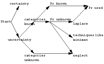
Hornby (1985) defines ‘risk’ as: “(instance of) possibility or chance of meeting danger, suffering loss, injury, etc.” Also: “at the ~ risk of / at ~ of, with the possibility of (loss etc.)”.

Thus, if there are possible outcomes O = {o₁, o₂, ..., o_n}, then the situation is risky if at least one of the o’s represents a loss. The risks are the o_i that are losses, thus Risks[O] = {o_i O | o_i is a loss}. The risk factors are the positions or index numbers of the risky outcomes, the i’s, or the dimensions (the causes that make such positions to be filled).

We will use the term ‘valued risk’ when a risk is valued with money or utility. When all risks have been made comparable by valuing them, then we can add them, and we will use the term expected risk value for the expected value of the ‘valued risks’. Then, crucially, once these definitions are well understood, then we may also use ‘the risk’ for the expected risk value. [110]

With such understanding, risk will be r = -E_x_<0[x] [111] or for short r = -E[x < 0]. [112]

Valued risk deals with the cases when probabilities are known or when unknowns are assumed to be uniformly distributed over known categories. It is not customary to use the term ‘risk’ for unknown categories. For example, it is uncommon to say, or write economics papers about this, that “all our lives are at risk of a suddenly imploding universe, or black hole hitting Earth, or waking up as a cockroaches”. Such real ‘Acts of God’ are commonly neglected. Note though that it still remains possible to say that a situation is risky even though one cannot put a number to it. Above expectation may be indeterminate since one may lack knowledge about the probability distribution or even the categories.

Relative risk is defined as r(t) = t - E[x < t] for some target level t. Risk (or absolute risk) takes t = 0, and relative risk would allow for a different target level. [113]

An interesting application is when x is a stochastic rate of return and r the certain rate, so that there is relative risk r(r) = r - E[x < r]. This relative risk answers the question: What is the probable loss with respect to a target return of r ? Here, r - r(r) = E[x < r] gives the weight of underperformance in the total target return (which weight has to be compensated by probable profits to achieve the target).

Conditional (relative) risk is defined as k(t) = t - E[x | x < t] for some target level t. With respect to rates of return, conditional risk k(r) answers the question: What would one expect to lose with respect to r, if earnings actually underperform and fall below r. Indeed, r - k(r) would give your expected return when actually underperforming.

Conditional risk is related to relative risk by the property that E[x | x < t] = E[x < t] / Pr[x < t]. The probable loss thus is corrected for the probability of the loss. Or, the probability measure in the expectation is corrected so that a density is taken that sums to 1. [114]

Example

In everyday parlance, profit and loss are nonnegative concepts. For example, if the difference between revenue and costs is $-10, then your loss is $10. It is only in mathematical economics that profits are defined as a general profit function such that ‘negative profits’ are possible. To understand risk, we however return to the everyday parlance convention.

Let us have a prospect that can give profit with probability p, and loss with probability 1 - p. We denote this as Prospect[profit, -loss, p]. We call profit * p ‘probable profit’ and loss * (1 - p) ‘probable loss’. Then the following definitions apply:

· Expected Value = = p profit + (1 - p) (-loss) = probable profit - probable loss

· Risk = risk value = expected value of the risks = probable loss = (1 - p) loss

· Risk Ratio = Risk / (ExpectedValue + Risk) = (1 - p) loss / (p profit)

· Thus: Expected Value = p profit (1 - Risk Ratio)

· Risk Probability = cumulative probability of all losses (in this case 1-p)

Risk is the (absolute value of the) down side of a bet. A venture is judged to be risky if the probable loss is large. Note that this notion still is somewhat vague. A probable loss can be large because of the probability or because of the sum of money involved. This vagueness is unfortunate, in some respects, but here is little to be done about it, since this vagueness is inherent in working with probabilities. In fact, this vagueness is an essentially positive aspect of working with probabilities. For, when we have different prospects, then we can order and evaluate them on risk, neglecting differences in losses and probabilities.

Colignatus (1999, 1999a) further develops these notions for simple binary prospects, multidimensional prospects, joint prospects, and continuous probability densities. An interesting application is the ‘Markowitz efficiency frontier’, but now with risk rather than the spread.

Wrong use in economics 1921-2005

The above definitions are proper in the sense that they conform to every day parlance and the definitions provided by Hornby’s dictionary op. cit.. The definitions provided here however differ from the use within the economics literature. First there are the definitions of Knight (1921) that have been adopted widely in economics, as for example in The New Palgrave (1998:III:358). Or it has become custom in finance to associate risk with the standard deviation. And some mathematical statisticians use another concept of risk. Let us discuss these in turn.

Uncertainty and risk

The New Palgrave, Eatwell c.s. (1998:III:358), gives the current common view:

“The most fundamental distinction in this branch of economic theory, due tot Knight (1921), is that of risk versus uncertainty. A situation is said to involve risk if the randomness facing an economic agent can be expressed in terms of specific numerical probabilities (these probabilities may either be objectively specified as with lottery tickets, or else reflect the individual’s own subjective beliefs). On the other hand, situations where the agent cannot (or does not) assign actual probabilities to the alternative possible occurences are said to involve uncertainty.”

Indeed, most economic texts use this distinction in this manner (at least, up to now). However, I cannot disagree more. The objections to Knight’s concept are:

(a) Certainty and uncertainty are binary. So, if a situation is not uncertain, then we have certainty, and there is no assigning of probabilities.

(b) If I am uncertain about a situation and assign equal probabilities to all cases - the Laplace suggestion - then according to Knight this no longer is uncertainty!

(c) In Hornby’s definition, the distinction is not between known and unknown probabilities, but the distinction is between events and human thought.

Figure 41 contains a diagram of the objectionable use of terms 1921-2005.

Figure 41: A diagram of the current but objectionable use of terms

The diagram clarifies the inconsistency with the binary character of certainty/uncertainty, the curious treatment of “Laplace”, and the over-use of terms by introducing the term ‘risk’ where there already is the qualification that the probabilities are known.

Risk is not the variance

The finance literature often uses the term ‘risk’ for the variance or spread (standard deviation) of the distribution of the rates of return of investments. This would be an improper use of the term. Suppose that one has a very profitable venture without the possibility of a loss. Suppose that the rate of return of this venture has a large variance, from mildly profitable to highly profitable. Is this a risky venture ? No, not in the usual understanding of the term.

Risk is not the negative of expected revenue

In mathematical statistics, some authors, like Ferguson (1967), define ‘risk’ as ‘expected loss’. However, it appears that they actually regard ‘loss’ as the negative of total returns (i.e. - revenue), so the definition used is -(p profit + (1-p) (-loss)), which is the negated expected value. This use of the term ‘risk’ is inappropriate. My proposal is to use the word “due” to stand for the negative of expected value, so that the standard statistical decision theory (with the game against nature) can be described as minimising due.

Note on Bernstein’s “Against the gods”

I came across Bernstein (1996) “Against the gods”, and found it equally entertaining as his “Capital Ideas”. One comment is that Bernstein indeed emphasises Knight’s and Keynes’s statements on “uncertainty”. My answer to that is, again, that unknown probabilities or even unknown categories indeed are serious cases of uncertainty, so that earlier writers on the subject were right in emphasising that seriousness. However, we should not be tempted to reserve the word “uncertainty” to only those cases. So with all due respect to Knight and Keynes, the definitions provided here are the proper ones.

Note on Wilson & Crouch (2001)

Wilson & Crouch (2001), “Risk-benefit analysis”, adopt the same definition of “risk” as discussed here. I saw this only after the first edition of this book. Since professor Wilson has been teaching on the subject for decades and his book only collects his teaching material I apparently only rediscovered what was already clear to him. Perhaps my presentation is a bit clearer since I use the formal E[.] notation. This chapter remains useful since it clarifies the confusions from the other definitions. Where risk is the product of probability and severity, this book also benefits from the emphasis on this definition, since, where I started to develop this argument after the Fall of the Berlin Wall in 1989, we have to deal with a future where there are huge dangers: though with only a small probability but on balance a relevant risk.

Book IX
Reduced form

39. The possibility of full employment in the welfare state

Introduction

Above we noted that the structural form of western welfare states is quite complicated. We would like to have a more enduring result than awareness of complexity, and therefor we adopt the Definition & Reality methodology. As said, a proposition - as a statement on reality - can be regarded as a mathematical theorem about/within a model of stylized facts. When there is a tautology, we attain truth by definition. So we now (a) restate what we consider to be the stylized facts, (b) define our concepts, (c) develop theorems and proofs, (d) link back to conclusions about reality.

The reduced form that is most relevant concerns the (long run) comparative statics of the regimes of full employment (1950-1970; Japan/Sweden) and unemployment (1970-2005).

This kind of comparative statics should not induce us to think that we abolish dynamics, though. Stagflation has both a dynamic (inflation) and a static or stationary (unemployment) aspect. When we skip proper dynamics and discuss regime switches in which unemployment features as an important switch variable, then Phillipscurve processes are included in the switching process, even though they don’t feature explicitly in the reduced form.

To attain the necessary level of generality, we use a reduced form where the economy is mapped into a model with three types of agents. One type is the net receiver; and two types are net tax payers. Since the latter two points give a line, that single line represents the state of the economy. The regime switch depends upon the choice of tax parameters.

Stylized facts

There are regimes of full employment (1950-1970; Japan/Sweden) and unemployment (1970-2005).

In the welfare state, it is more efficient to have full employment. Unemployment causes lower income - not only directly as in old-fashioned capitalism but also, more noteworthy, by the additional benefit burden. Unemployment can have an adverse effect on inflation when it causes a shift of the Phillipscurve.

It turns out that the propositions that are most interesting, from the viewpoint of political economy, do not require continuity, and can be formulated by assuming dichotomous High and Low productivity labour, combined with one class of Benefit recipients. This assumption allows for a reduced form formulation that allows for generality. For expository reasons we can take social subsistence and productivities as purely constant. In the simple mathematical model the dichotomy gives fixed numbers, in actual observation they are subgroup averages which depend upon general equilibrium processes. The benefit level is rather not an average but a threshold, like the surface of the sea at Scheveningen beach. The words Benefit, High, and Low give letters BHL, and this abbreviation may be pronounced - converged upon after many walks - as ‘beachly’.

It is a stylized fact that welfare states are BHL. Checking this requires next definitions.

Concepts

Here we will redefine variables such as H, Z, b, n etcetera. Also the reduced tax function will be T(.) as opposed to structural T[.]. These redefinitions hold for this chapter 39 and chapter 40 - that together form a reduced form unity.

Definition: Biological subsistence, for survival, is S.

Definition:       An economy is a welfare state iff people without income are not left to charity, stealing or death, but get a benefit B. The benefit B has the following properties:
i.           the net benefit has the social subsistence level B S,
ii.          people on benefit may not work, [115]
iii.         eligible are:
iii-a.      permanent benefit recipients (e.g. ‘the elderly’)
iii-b.      people able to work but currently unable to earn at least
             net B (these people are called ‘the unemployed’).

Remark: it is useful to have category (iii-a) in the model. It introduces a degree of sufficient complexity. When there are levies even under full employment, then it is easier to understand that wrong co-ordination may cause a switch to unemployment. But (iii-a) might count zero people.

Remark: Property (iii-b) has the effect of a legal minimum wage. It sets a floor in the market. We might introduce a benefit threshold (for workers) XB such that S XB < B, but for expository reasons, we take XB = B.

Remark: The reservation wage effect is as follows. When vacancies with net income higher than B are registered, then the relevant unemployment benefits are simply scratched. This mimics the array of measures needed for continuous reality.

Remark: This definition implies that people working with subsidies in the Swedish/Japanese case are not on ‘benefit’. Such subsidies thus must be accounted differently, basically as part of taxes.

Remark: The black economy (another form of working while on welfare) is neglected. We neglect also the case that some people hate being on welfare, and thus continue working even when their net earnings are below the benefit threshold (S < net earnings < XB ).

Definition: A welfare state is bhl iff it remains meaningful to trisect its membership into the economic classes of Low and High productivity workers and permanent Benefit recipients.

Definition: A welfare state is nonrevolutionary, iff its economic classes and their data are stable across the change of employment regime.

Definition: A welfare state is BHL iff it is bhl and nonrevolutionary.

Remark: Denote High and Low gross productivity as H and L. Note that B is net. Also bhl-ness technically implies H >> L B.

Remark: L may be associated with a minimum wage and H with some average income including profits.

Remark: An example of ‘meaningful’ are subgroup subperiod averages.

Remark: Stability can sometimes be found by normalizing, e.g. take subperiod H(t) as the subperiod numeraire.

Remark: A person’s benefit is often related to the former period working wage. However, anything can be clustered into a social subsistence average. People ‘between jobs’ could be taken to be basically in the employed cluster, people with serious unemployment could be in the other cluster. Don’t object that this makes the matter tautological - since that is exactly what we try to do. (We try to find the definitions that make our understanding tautological.)

Remark: A nonrevolutionary welfare state still allows for politics and economic change.

Lemma I: A welfare state is BHL iff there is stability over the regimes for the variables B, H, L and the associated numbers of agents.

Proof: Self evident. Q.E.D.

Remark: The relevant notion is that the change from unemployment towards full employment (or vice versa) does not destroy the productive base of the economy. Instead of taking this notion explicitly, we have taken a stronger property of nonrevolutionarity, that allows, if bhl-ness applies too, to take (approximate) constancy of the variables.

Remark: At first glance these definitions seem self-defeating for the effort to apply the mathematical method to employment regime switches. When 35 million, nowadays unemployed in the OECD, are supposed to find a job, then apparently the policy maker is supposed to be able to judge on the ‘stabilities’ involved. That seems an impossibly strong assumption. We may however remind about the regime switch from 1950-1970 to 1970-2005. In addition, as modellers we discuss equilibrium states of various paths. Also, it is possible to give the variables an incremental interpretation, e.g. take 34 of the 35 (million) as permanently on benefit, and only look at 1 million on the margin (giving “local-BHL-ness”).

Lemma II: For a welfare state, the (apparent) existence of people with a productivity L’< B, does not block the application of BHL-ness.

Proof: Consider the pathological case of people with productivity L’< B, i.e. so low that (in whatever regime) their net market income is lower than B. Take the dentists, who in a regulated market cannot start a practice, and who are very bad at farming in a flowerpot (which could be done with a Cobb-Douglas production function). These people can be treated as:

(1) society is willing to classify them as (iii-a)

(2) like the Swedish/Japanese approach, they may keep on working with some employer subsidy Z; in that case L = L’ + Z

(3) society lowers B to B = S or B = L’, and reconsiders the problem

(4) if regulations are the bottleneck, then changing these regulations redefines ‘given’ productivity L’. Similarly, if Keynesian methods solve unemployment, then only if people’s effective productivity is restored. So the reduced form applies anyhow. (In that case the regulation or lack of a policy measure is a tax in terms of the reduced form, and ‘real productivity’ is higher than L’.)

(5) they get charity, steal or die, and hence there is no welfare state.

Hence BHL-ness implies that these cases can be ‘averaged out of the discussion’ or be left out for expository reasons.

Q.E.D.

Remark: In other words, BHL-ness is sufficient for discussing employment in the welfare state (but not necessarily for other topics, for example, how regulations affect productivity).

The theorem

Theorem BHL.1: For a BHL economy, both full employment and unemployment are possible.

Proof:

The structure of this proof is, that we determine the accounting equations, find the reduced form tax relations that are implicit in these, and then deduce the critical tax parameters that determine the regime switch.

Looking at the BHL concept, the only possibility for variation is in category (iii-b). The recipients in that class all move together, and thus there are only two regimes (in or out of benefit dependency). Given that gross productivity has been fixed, the only possible variation concerns net income. We assign the term “tax regime” to the possible states in net income. We find, in other words, that these regimes are implicit in the BHL concept. Let t be the index for tax regime 0 (unemployment) or 1 (full employment).

Given BHL-ness, we thus have: t is 0 or 1, and:

b permanent benefit recipients;

h persons with gross productivity H and net N(t);

l persons with gross productivity L << H, and net K(t).

The regimes are characterized by net income conditions K(0) < B and K(1) B:

(0) In regime 0, K(0) < B and l are eligible for benefit B, and they don’t work.

(1) In regime 1, K(1) B and l don’t get benefit B, and they work and earn L.

On benefit, the welfare rule is strict on not-working, while by assumption the black economy can be neglected. Off benefit, the l have no other means of support and thus work, and earn gross L. Since net income cannot be larger, L K(1) B.

In the following equations, personal income y takes values H and L. Relation (1-t) below gives the implied tax system, where the personal tax T(y, t) depends upon personal income y and the tax regime t:

T(H, t) H - N(t) ; T(L, t) L - K(t) (1-t)

Two points share a line. Hence, the tax system can be represented by a straight line, with an intercept and a marginal tariff. These implied ‘parameters’ (actually: reduced form variables) are defined in (2-t), with 2 pairs of 2 equations & 2 unknowns, giving tax exemption X(t) and marginal rate R(t). The line is the reduced form representation, while the statutory system which guides people’s actions could be anything. Each regime gives a set of reduced form lines; our interest concerns the boundary line.

R(t) (y - X(t)) T(y, t) (2-t)

Relation (3-t) defines national income Y(t), where the personal incomes are multiplied by the numbers of persons involved. Revenues h H + b 0 = h H are regime independent. Depending upon the regime the l bring in L or not.

Y(t) h H + t l L + b 0 (3-t)

Relation (4-t) states the condition of a balanced budget. National income equals the sum of net incomes after redistribution. The condition may be called “Walras’ Law”.

Y(0) = h H = h N(0) + (l + b) B (4-0)

or h T(H, 0) = (l + b) B

Y(1) = h H + l L = h N(1) + l K(1) + b B (4-1)

or h T(H, 1) + l T(L, 1) = b B

The budget condition implies that the tax ‘parameters’ are functions of each other. Per regime, a higher exemption means a higher marginal tariff, and vice versa. The regime switch itself might, but need not, be the exception. Given that marginal rates R are generally regarded as policy variables, we solve for X. With X(1) L:

(4-0) h R(0) (H - X(0)) = (l + b) B

X(0) = H - (l + b) B / (h R(0)) (5-0)

(4-1) h R(1) (H - X(1)) + l R(1) (L - X(1)) = b B

X(1) = (h H + l L - b B / R(1)) / (h + l) (5-1)

There is a set of critical levels of gross income M(t) = M(R(t), t), such that unemployment results iff earnings L are less than M(t). This follows directly from rule (iii-b). This critical income solves from:

M(t) - T(M(t), t) B

M(t) = M(R(t), t) = (B - R(t) X(t)) / (1 - R(t)) (6-t)

Under unemployment, the benefits cause additional taxes l.B which are levied on a smaller tax base. Given that l are unemployed anyway, the tax exemption X(0) can be lowered, so that the marginal rate is as low as possible. This has the effect that M(0) shifts to the right, so that the gap between the possible wage L and the wage ‘required for a decent living’ widens. There is obviously hysteresis, of a ‘catastrophic’ kind. Conversely, M(1) can range in B M(1) L and allow for larger R(1) though this could have little effect since also X(1) rises (see below). While these properties apply to the reduced form, the same mechanisms apparently apply to the structural form too (as they concern the same reality).

Substituting (5-t) in (6-t) gives M(t) as an explicit function of R(t). The regime switch occurs at M(1) = M(RS, 1) = L with switch marginal rate RS and implied exemption XS:

                                        bB - (h + l) (L - B)
                        RS =     -----------------------------                                  (7-RS)
                                             h (H - L)

                                        bB - (hH/L + l) (L - B)
                        XS = L   ----------------------------------               (7-XS)
                                           bB - (h + l) (L - B)

Rewriting conditions K(0) < B and K(1) B gives:

{L - T(L, t) < B} { X(t) XS & L < M(t)} (8-t)

{L - T(L, t) > B} {X(t) XS & L > M(t)} (9-t)

Now consider the regimes, and determine whether they can exist:

Full employment: Given that L > B, it follows from (9-1) that the tax exemption can be chosen on or above the critical value XS. Hence XS X(1) < H. A prime example is X(1) = B. Hence (iii-b) is empty.

Unemployment: L is given as the market clearing wage for low productivity persons. If X(0) < XS, then taxes on these persons are increased, and their net income drops below B. Given that K(0) < B, they are eligible for benefits, and apply. Hence (iii-b) is not empty.

It has been shown that both cases are possible. Q.E.D.

Remark: This exposition may seem an overly complex translation of the Cohen Stuart 1889 quote (above) to the welfare state situation. The proof might have said “self-evident” after the first paragraph. Given the record of unnecessary unemployment, this author may however be excused for driving the point home. The usefulness of the BHL concept may be, that officials now can report, “we have diagnosed l people on benefit who should be able to earn L > B on the market, so let’s try to find out how we are stopping them from doing so”.

Remark: A more didactic exposition may start with a structural tax relation, e.g. with R(t) replaced by r in (2-t); see for example the Bentham tax. Then one can show that a ceteris paribus reduction of the tax exemption will increase unemployment. Hence, for the return of full employment it is necessary (but not sufficient) to increase income tax exemption - or something from the ceteris paribus part. Then, the second step in the exposition (as we have done here) is to rename the axis into compounded variables (including VAT, regulations, subsidies, excises, charity, etcetera), and then consider (2-t) as the reduced form. Then we find necessary and sufficient conditions. This however only works satisfactorily for an accepted model of a real economy.

Remark: The theorem doesn’t establish that unemployment has only one cause. Various kinds of unemployment have various causes. But, when various causes are mapped into the world of BHL-ness, then the theorem applies. For example, a long term unemployed academic would be categorised as unskilled labour, even though his employed colleagues earn much more. (The BHL concept thus is drastic. The reasons for applying it have been explained elsewhere.)

Remark: The theorem is strongest in the t = 1 t = 0 part. Given full employment, it is easy to mess it up; and it is easy to see that you can mess it up. The other way around is less obvious. Here, both the requirement L B and Lemma II are crucial. For expository reasons those are sufficient, but not as sharp as they could be. For example, we might accept a small loss in H(1) H(0), as long as net N(1) N(0).
However, even then the analytical structure remains, that productivity L is assumed, so that it doesn’t come as a big surprise that employment is possible. This actually is similar to the Arrow-Debreu setting, where endowments are assumed, and full employment appears to be possible. The modern reader might be inclined towards assumptions that generate the impossibility of full employment. (See for example the Grandmont (1983) setting of expectatory mismatch.) However, each impossibility can be questioned too. It is up to reality what model applies. Stated differently: the value of above tautological theorem is that it helps us to understand what is implicit in our concepts, so that we may be more aware in observing whether these concepts apply. This fits in with our concept of a proposition.

Remark: The reduced form also captures the ‘physical tax’. The lack of infrastructure, machines or tools may ‘tax’ people - and once these have been provided, they could start earning income, and their earnings would, crucially, be larger than needed to pay for the equipment. Economists of course understand this concept of a physical tax - as the lack of efficient capital markets, or the frustration of those by taxes - but the crucial point is the abstract one. When people don’t earn anything, and the economist suggests to abolish some tax, then a listener may become upset, since how can you abolish something that people don’t pay ?

Graphical presentation

Diagrams help understanding the analysis. Figure 42 shows two tax regimes, T(y, 0) and T(y, 1), characterized by different exemptions X(0) and X(1), and different critical incomes M(0) and M(1). The main difference is net income at L. In regime 0, net income at L falls below subsistence, causing unemployment and higher taxes to pay for benefits.

Figure 42: Tax regimes

It can be seen that T(y, 0) is above T(y, 1), or that average tax rates are lower under full employment. On the left section of the horizontal axis, X(0) < X(1). On the right section, since taxes in regime 0 are higher and levied on a smaller tax base, T(H, 0) > T(H, 1). Thus the effect on the average tax rate is clear. The effect on the marginal rate depends upon the numbers. The case depicted here, with a higher marginal rate in regime 1, is only one possibility; but it shows that a higher marginal rate can combine with actually lower taxes.

40. The possibility of co-ordination

Chapter 40 showed the technical possibility of full employment for a welfare state. Chapter 34 showed that social choice is feasible, in the sense that there are consistent and reasonable constitutions that society might deem attractive. In particular, there is the example of a constitution that uses the efficiency criterion (Pareto optimality, PO) to select its policy. There still remains one issue to settle. This is the issue of information. Society might have a consistent preference, and consistently prefer full employment above unemployment, but when people don’t know that it is possible, and instead even have theories that tell them that full employment is impossible, then society might still choose for unemployment as the best of all evils. The issue of information already featured in our discussion of Arrow’s Theorem, and now returns for our discussion of unemployment.

We again follow the procedure given by our methodology. We select stylized facts, develop our concepts, deduce results, and link back to reality. We will first construct a subsidiary lemma that is very general and concerns any suboptimality due to misinformation. Then we take our theorem on the possibility of full employment, recognise it as an item of information, insert it, and construct our theorem on the possibility of co-ordination. [116]

Stylized facts

Recorded full employment situations may have been caused by ‘chance’. Policy makers in 1950-1970 may have thought that functional finance was effective, while it also was the tax exemption level. A re-evaluation of the history may however also show that leading economic advisers in the 1950s may have been wiser than those of the 1960s.

It remains a stylized fact that much of the subject matter on employment is well-known. For example in Holland, CPB economists Van Schaaijk (1983), Bakhoven (1988) and Colignatus (1990) pointed the way to full employment. The state of knowledge turns out to be part of the model.

There is a Pareto Optimizing Change (POC) iff some advance and none suffer. A change from unemployment to employment need not be strictly POC. Note that we already have resolved that we don’t need high unemployment to keep inflation in check. So the CWIRU is no argument against a POC. There are other clear reasons that pose a problem. First these two:

· Some bureaucrats have plush jobs administrating the unemployed, and would lose their job and sense of power.

· The unemployed would lose their leisure. For some, the combination of low benefit B and leisure might be preferable to work at a higher income.

We can overcome these barriers by going back to basics, i.e. to our definitions. First of all, the bureaucrats are reminded that they are there to serve the public cause (‘res publica’) - and thus they have signed a contract - before they got the job - that they will welcome full employment and raise no anti-POC objections. In the same way, the people on the dole have signed a contract - before they got the benefit - that they will accept a job at a living wage, and will not raise anti-POC objections either.

A final observation is that the power elite, those who determine the SWF, might enjoy unemployment of a section of the population for some strange other reason. They might not care about the increase of income, freedom and welfare from a change towards full employment, but they would prefer the idea of people in helpless positions and the warm gratitude they show for their benefits. A king needs subjects. We resolve this problem by proper formulation of the theorem.

Concepts

Note that we use the symbols of chapter 39 (that forms a unity with this chapter).

Above theorem on the technical possibility of full employment is essentially incomplete. It has not been specified how the tax regime comes about. The tax regime is an expression of the social choice already made, but it has not been explained how a particular choice has been caused. What is required is a power distribution on the b + h + l agents in the economy. In conventional terms the power distribution is expressed as a social welfare function SWF, and the tax regime is the result of the maximisation subject to the state of information I:

maximise SWF(h, H, N, l, L, K, b, B, t; I) (40.1)

Using a SWF serves expository purposes. When turning to practical application we could use the Drissen & Van Winden (1990) approach. But the logic of both approaches is the same.

The introduction of regime indicator t as a separate variable in the SWF means that it stands as a proxy. The economy is not simply a collection of individuals maximizing utility over consumption and labour. There are some institutional aspects too. An example of an institutional influence is that some social security officials might benefit from unemployment, since it keeps them in attractive jobs. All such (Public Choice) phenomena can be collected on their point of relevance: the employment regime t.

Secondly, there is information I. Ever since Keynes and Tinbergen, or even earlier, but for some economists more acutely since Muth and Lucas, economists have given attention to the information sets that guide the activity of agents. This concerns not just plain knowledge, but rather what people believe about the state of the world. The information sets may contain individual and social aspects, like own prices and the (announced) general price level.

Variable I is an aggregate. It represents the state of knowledge of those in power, where ‘having some power’ is a state of nature given by an array or by a distribution. The latter is not further developed here. A basic point however is that if some economist would know how to solve unemployment, but those in power don’t, then the budget set is I_B, while I < I_B - and those in power apparently prefer not to know. [117]

The use of variable I could complicate the analysis in various ways. R&D could be an economic activity affecting social welfare itself, amending (40.1) etcetera. But the present formulation suffices for our purposes. Note, the maximisation process itself finds its operational implementation in the actual work of some agents in the economy. Such work might be implicit and thus not explicitly remunerated. More conventionally there are some administrators (e.g. a “Council of Economic Advisers“) who are explicitly paid for their information handling activities (often: whatever outcome on t).

Piore (1987) reminds us that unemployment is not a natural disaster like an earthquake, but derives its cause, nature and significance from the social system as a whole. In this line, when unemployment arises, we would find the solution by studying the whole system. This includes information. And Piore’s reminder, being a reminder, is a piece of information. Indeed, one important social type of information concerns theory itself, and economic models in particular. The development of the theory of Rational Expectations (or model-consistency) implies this too. Economic theories about unemployment are themselves part of the information sets in society. An adequate description of unemployment not only requires a statement of taxes, social security and e.g. legal minimum wage, and their technical interaction, but also a statement of people’s perceptions, of the theories in the journals, and of what journalists and politicians make of these.

When unemployment arises, it may be caused by the power distribution, but the cause can also be plain lack of knowlegde. It may very well be that Piore’s proposition has not gotten sufficient attention from policy makers and advisers. And this lack of attention, if it were true, would be a prime example of the influence of the information set on economic activity.

There are two relevant states of information: I = 1 meaning that those in power perceive of a (sound, compact) solution of unemployment, and I = 0 meaning that this is not the case. Note that knowledge about the theorem on co-ordination, that is to be formulated next, might but need not be included itself in I = 1.

The Dissipation of Knowledge I by science, education and media need not be detriment to those in power, but it might be. In the latter case I would not be POC in the ordinary sense. However, many would hold that I morally dominates POC - and if these people are in power, then this conviction is reflected in the SWF. Note also that I need not be positive, e.g. when a wise king dies or a wise government party loses the elections. Note that when I coincides with a shift in power, the prime cause can be both personal properties involved or the information; but here everything is aggregated into the latter.

We conclude this section by a short abstract discussion of the concept and properties of information, and Lemma III.

Regard a controlable dichotomous system with states s = 0 or s = 1. Two consecutive states are of the form {0, 0} and {1, 1} where the regimes are maintained, and {0, 1} and {1, 0} where there is a switch. If policy is conscious, then the movement from one state to the other (or the same) depends on information - and thus there are four lists of basic information. With 4 such items, an agent’ mind can possess any combination. There are 15 of such combinations: namely 1 case where all 4 are known, 4 cases of only 3 items, 6 of 2 items, and 4 cases when only 1 is known. It will be useful to compress this abundance.

The following definitions are useful:

Definition: Basic information is a list of “what one does” to have one state in one moment and another state in the next moment. An example list is: {“Provide oxygen and a dry place”, “Light the match”, “Let it burn till it is all cinders.”}. Other examples are recipes, film scripts, computer programs (“Click on a button”). We can denote basic information as BI(s₁, s₂). Note: In this version of the proof we allow basic information to be true or false.

Definition: A state s is said to be controlable iff there exists - in principle - true basic information on both s and 1-s, and the agents have the resources to use this information. Note that this information need not be known by the agents (need not be available), and it need not even be known to the agents that the matter is not unknowable.

Definition: Information is available when at least one agent in the economy has it. (This is stronger than the ‘existence in principle’ of controlability.)

Definition: Sound information J(s) is a list of both what one does to maintain s and what one might do to change s into 1 - s, using true cause and effect relations. Thus J(s) = BI(s, s) BI(s, 1-s) | truth. Denote an arbritrary belief as J’(s) - that however will not be sound since it would not be necessarily true.

Remark: True information is sound when the information concerning {1, 1} and {1, 0} is joined, or if the information on {0, 0} and {0, 1} is joined. One may e.g. know how to burn or not to burn a match, but not how to restore cinders into a match again (except for restarting the universe, but that is not likely controlable). Let 1 stand for match, and 0 for cinders. Then J(1) exists, but J(0) doesn’t (only partly, to maintain cinders as they are). Using sound information rather than basic information has analytical advantage. A Roman emperor may think that he maintains his good fortune by sacrificing to the gods. We rather discuss cases where governments deliberately abstain from wrong policies.

Remark: Consider the list {“If you happen to flip back to 0, use BI(0, 1) to go back to 1”}. Can we classify this as BI(1, 1) ? We could allow this if the cost of the temporary flip is low. For example, riding a bicycle requires continual readjustment of equilibrium. We can define BI(s, s) = {chance(s, 1-s)} BI(1-s, s) | truth, as implied control information. But since this does not give BI(s,1-s), the implied control information does not give sound information. Stated differently, we are interested in durable states s, and not in flipping states. If we observe s then we want this to be caused by deliberate rejection of the use of BI(s, 1-s). We also regard cases in which implied control would be costly.

Definition: The tuple (J(1), J(0), s) is the state of a sound system. Note: Though the information is denoted as a function of s, information in a controlable state is the prime cause and s the prime effect.

Definition: Information is called compact iff J(0) J(1). Note: Compactness means that one knows the explanation of one state, iff one knows the explanation for the other state. Then we can use a single variable J or J’.

Definition: A state s is said to be caused by chance iff a situation of s and unsound belief J’(s) are stable. It is said then that there is a hidden cause linking J(s) to s.

Definition: If the sound information concerns a model then we can denote J in binary values, with 1 = ‘the model is known’ and 0 = ‘the model isn’t known’, rather than use the whole list of statements. With binary information, compactness J(0) J(1) becomes J(0) = J(1).

Remark: Consider the example of the Roman emperor. His model is ‘sacrifice fortune’ (and if fortune slips after a sacrifice, then apparently more sacrifices are required). One of his basic informations is BI(~fortune, fortune) = {‘sacrifice fortune’, ‘In this case sacrifice’}. Since J’(1) J’(0) this is a compact belief.

Remark: If s is the case, and one doesn’t believe J(s), so that J(s) = 0, then one believes some alternative J’(s). Someone unfamiliar with matches would have the unsound (perhaps only basic) information ‘this is just a piece of wood’. More complex situations need thorough analysis. E.g. someone may know the text of a theorem and benefit from that, but may not know its proof.

Lemma III: If there is sound information (J(1), J(0)) on a controlable dichotomous state s, then:
(i) if the information is not compact then there are 8 states of the system, with 4 states implying a hidden cause,
(ii) if the information is compact, these numbers are halved.

Proof:

We tabulate the possible states of the system (J(1), J(0), s) in Table 16.

In cases (rows) (3), (4), (6) and (7), the agent doesn’t possess sound information and believes some J(s) (e.g. ‘the world is as it is’), but he chances at s nevertheless. This implies that there is a hidden cause. (For example, the state of the system was inherited, and the agent wishes to keep things as they are. In that case (J’(1), J’(0), s) has causality within a more complex model, describing in more detail how people act on their beliefs.)

If the information is compact, we only consider states (1) to (4). Q.E.D.

Discussion: To understand the proof, look for example at row 6: There is a true model for sequential states {1, 1} and {1, 0}, or to maintain 1 or change to 0. But nothing is truly known about maintaining 0 or changing back from 0 to 1 (though beliefs can exist). Observed is s = 0. Perhaps it once was a conscious choice to go from 1 to 0, and perhaps one uses the implied control {chance(0, 1)} BI(1, 0) | truth. But we are concerned with durable cases for which implied control would be costly. We want to see deliberate rejection of the use of BI(0, 1). But this information is not present. Hence the endurance of 0 is caused by chance.

Table 16: States of the system

	J	J(1)	J(0)	s	meaning
(1)

The Project Gutenberg eBook, Definition & Reality in the General Theory of Political Economy, by Thomas Colignatus

Definition & Reality in the General Theory of Political Economy

Book I Introduction

1. Order of presentation

2. The general theory

3. Methodology

Book II Trias Politica and Economic Supreme Court

4. The Trias Politica

5. The economic record of the 20th century

6. An Economic Supreme Court

7. Position of the Court in economic theory

8. The record of economics itself

9. Economics ‘as usual’ and its inadequacy

10. Four empirical cases

11. The moral imperative

Book III Economics ‘as usual’

12. Introduction

Stylized history

Structure of the argument

The difference that it means

13. Unemployment via taxes and minimum wage

The earnings distribution

Analysing the minimum wage

The Tax Void

Cause of the Tax Void

Taxes

Subsistence

Deduction of the real net average income index

When all incomes grow as fast

Development of the Tax Void

Graphical presentation of the Dutch data

Using the data for our analysis

Marginal tax rate & VAT

Marginal tax rate & dynamics

Spillover and domino effects

Diagnosis and Therapy

Stagflation resolved

14. The 1974 Duisenberg disaster

Book IV Presentations for the general public

15. Unemployment solved !

16. Enable Russia to help itself

Parallel

Risk not chance

Internal not external

Conclusion

17. Will the West repeat Versailles ?

Book V Methodology: Definition & Reality

18. How to check ?

19. Dealing economically with concepts

Maximising information power

Pythagoras and the circle

Falsification

Determinism and free will

From stylized fact to definition

Relating to Hicks 1983

20. Structural and reduced form

21. Direct application to the Economic Supreme Court

22. Methodological summary

Book VI Structural models

23. A textbook macro-economic model

The IS-LM model

The production function

Dynamics versus statics

Phillipscurve

Macro-economic interactions

24. Heterogeneity and nonlinear taxation

Heterogeneity versus homogeneity

Nonlinear versus proportional taxation

Some literature

25. Summary of current views

A simple view

A complex view

Efficiency wages intermezzo

A more sophisticated view

Confusions

26. Heterogeneous labour

Dromedary supply

Dutch income distribution data

Definitions and formulas

Amendment to the textbook model on the Phillipscurve

Definition & Reality
in the
General Theory of Political Economy

Book I
Introduction

Book II
Trias Politica and Economic Supreme Court

5. The economic record of the 20^th century

Book III
Economics ‘as usual’

Book IV
Presentations for the general public

Book V
Methodology: Definition & Reality

Book VI
Structural models

Book VII
Social Choice